13 Assembly
13.1 Vectorization
It is convenient to introduce the vectorization or flattening operation. Given a multidimensional array with indices, through , where the th index ranges from 1 to , we can associate each entry in the array with an entry in a one-dimensional array. The mapping of a multidimensional index to a single index is given by The transformation can be expressed in indexed form as a multidimensional array whose entries satisfy Note that changing the ordering of the indices in the subscript of the flattening array changes the ordering of the resulting matrix.
Consider the matrix The one-dimensional array produced by is Reversing the ordering of the flattened indices produces the following array In the two-dimensional setting, these correspond to the standard column major and row major conventions for storing arrays.
We represent mappings such as geometry and solutions by defining a set of coefficients and forming a linear combination of associated basis functions: If we use vector-valued coefficients drawn from a vector space with basis , then is an element of the vector space defined by the tensor product of and , . The representation of in terms of the basis for and the basis for is We can view as a trivial vector-valued function space having a basis given by and representing as a single sum: This is typically the representation employed in finite element analysis. Note that it is also possible to define the basis as . This provides an alternate representation and indexing for the same basis. We prefer the first indexing for improved locality of the coefficient data as all values associated with a single function from the base scalar space are contiguous in the array .
13.2 Scattering
We introduce the notion of a scatter matrix. Given an ordered set of indices chosen from where , the scatter matrix is the matrix having entries defined by If then is the identity matrix. We call this the scatter matrix because it scatters a vector of values into a larger vector of values with some zeros interspersed. The transpose of the scatter matrix could be termed the gather matrix because it gathers specific values from a larger vector into a smaller vector. Similarly, the scatter matrix and its transpose can be used to scatter a smaller matrix into a larger matrix ( for a square matrix ) or select from a larger matrix into a smaller matrix ( again for a square matrix ). If the parameter is obvious from context then it may be omitted.
The direct sum may be rewritten as a standard sum using the scatter matrix. We assume that the region identifiers are ordered and define the block index sets where . Then we have that where and .
13.3 Bases
We assume that the domain of our problem can be decomposed into subdomains that we refer to as regions. These regions are typically chosen to provide certain structure in the parameterization, basis, or related properties. Each region has an associated function space, . We typically define these functions spaces by choosing an appropriate basis defined over the region. Common examples include the polynomials defined over a unit interval (box) or the tensor product B-splines. We assume that the solution to our problem can be approximated as a member of the space formed from the direct sum over all function spaces associated with the regions of our problem domain:
The most familiar example of this construction is the function space employed in a standard Discontinuous Galerkin (DG) formulation. In this case, the regions are the elements of the mesh and the associated function spaces are typically selected to be standard polynomials over the elements.
It is often advantageous to restrict the solution to a subspace of that is smaller or better-suited to the problem at hand. This can be accomplished by defining a new basis formed from linear combinations of the basis of .
The most common example is a standard implementation of the finite element method with a basis of uniform degree. In this case, the regions are again the elements of the mesh and the associated function spaces are again chosen to be polynomials. We define a new set of basis functions as where . This is a basis for a new space, . The dimensions of the matrix are . If the basis used to represent the function space on each element is chosen to be a basis that interpolates the boundaries or a tensor product of bases that interpolate the boundaries such as the Bernstein basis or Lagrange basis, then the entries of the matrix are all ones with the sum of each row in the matrix being the number of elements adjacent to the topological entity associated with the function.
Given a mapping represented in terms of the basis of , we apply the relation between the basis of and to obtain and observe that by rearranging the sums, the matrix can be used to transform the coefficients of the mapping for the basis of into coefficients of the basis of : where the index ranges from to . This follows from the fact that is a subspace of .
We can also apply similar strategies to higher-order spline-based decompositions. While it is possible to choose regions to generate the same elements and basis as one would choose for a finite element space, significant benefits can be derived from a higher-level approach. Rather than decompose the mesh into individual elements, where possible, we choose regions of the mesh that can be represented as tensor product grids. This permits the representation of arbitrary meshes while leveraging any available tensor product structure. For each region, , the region function space , is chosen to be the space spanned by the B-spline basis constructed over the associated tensor product grid. We again define a region-discontinuous function space as While it is possible to generate region-internal discontinuities, the term “discontinuous” refers to lack of continuity across boundaries between regions. We define a continuous basis as a linear combination of the spline basis functions of the regions: The entries of the matrix can be computed by projecting the continuous basis onto the region subspaces or by applying the U-spline algorithm.
The spline space is the space spanned by , where is the number of columns (second index) in . This matrix is often referred to as a prolongation matrix and is intrisic to the choice of basis for the global function space and for the local subspaces. We’ve used the symbol to represent the prolongation matrix here, in the event that we need to distinguish between the test and trial basis we will use and to refer to the prolongation matrices associated with the test and trial bases respectively.
13.4 Bilinear Forms
We consider a problem defined by a bilinear form and linear form : where is an element of the test space and is an element of the trial space. The global spaces are formed from a direct sum of the region subspaces
We use to represent the th global test basis function and to represent the th global trial basis function. Inserting these basis functions into the bilinear form gives which can, in turn, be written in terms of the basis functions and of the larger spaces and , respectively, as
We now use to represent a test function in th region and to represent a trial function in th region and define the matrix We can then rewrite the bilinear form in matrix-vector form as
13.4.1 Active Scatter Matrices
Let be the set containing indices of functions in some space such that the image of the support of the function under the spatial map (associated with the region) has a nonzero intersection with the simulation part. We then construct the scatter matrices from the active index sets and insert them into equation which gives If we define the matrices and the vectors then we can write the linear system restricted to active entries as We generally want to form only the active entries of all matrices and vectors rather than the full system.
It is often possible to choose the tensor product regions that decompose the mesh to so that most of the scatter matrices are the identity. This is advantageous because zero rows in and correspond to work done to produce values that are not used in the final system. To simplify the exposition we will neglect to write the scatter operators and or the superscript . It may be more efficient to assembly tensor product regions and then remove the unused terms using the scatter matrix. For now, we will assume that all region spaces are restricted to the functions that overlap the part for simplicity.
13.5 Basis Extension
13.5.1 Section heading
Accurate and efficient solution of a flex problem often requires the use of extension operators and . Introducing the extension operator into the prototype equation produces
13.5.2 Section heading
We also define the compressed matrix, , associated with as
In a parallel setting it is often advantageous to compute the sparsity pattern of the extension operator from a minimal amount of information. We have determined that the minimal data required to compute the sparsity is a matrix representing the element-function connectivity and an array, , containing the interior fraction of each active base element. The element-function connectivity matrix, , has a row for each active base element and a column for each active base function. The matrix is sparse with a nonzero entry for each function that is nonzero over a given cell. The value stored is unimportant for the sparsity computation but it may be useful to store the value of the integral of each function over the associated cell for use in the construction of restriction operators.
It may also be best to store a sparse element adjacency matrix, , indexed by the element indices in each direction. This matrix is sparse with nonzero values indicating the interior area of the interface shared by the elements indexed by the row and column.
Elements are separated into generations. We represent the th generation with a vector, , indexed by the active elements. The vector entries associated with the elements in the generation are one, all other entries are zero. We require the generation matrices, The set of indices included in the th generation, is also useful.
It is convenient to define the set of elements included in a given generation, , and all previous generations, . We also define the complement of this set, that is all elements excluded from a given generation and any previous generations, . The associated matrix representing the elements included in the generation and all preceeding generations, , and the matrix representing the elements not included in the generation and preceeding generations, , enable us to express certain steps easily.
The construction of the extension operator sparsity begins with a choice of the cutoff value, for the volume ratio.
This value is used to form the initial generation vector: The subsequent generation vectors can be defined using the adjacency matrix . We begin by defining the link candidate matrix associated with the generation as where is a sparse matrix with a value of one for each nonzero entry in . The indices of rows of with nonzero entries are the indices of the elements in generation .
Another key component is the representation of generation links. This is most easily represented as a sparse matrix, , indexed in both directions by element index. Only rows associated with elements of the current generation, have nonzero values. Each row has a single nonzero value whose column index is associated with a element from a previous generation. This can also be stored as a list of pairs with the first value indicating the current generation and the second value indicating the link to a element from a previous generation.
A primary component of the construction of the extension matrix sparsity is the selection of links between the generation being constructed and previous generations. The first criterion is that links be formed with the earliest possible generation. In the event that multiple link candidates remain, the link is formed with the element having the largest shared interface.
It is helpful to define the generation weighting matrix, The first criterion can be satisfied by choosing the column indices on each row of the product whose associated values are equal to the rowwise maximum (excluding rows with no nonzeros).
The second criterion can be satisfied by choosing the column indices on each row of the product whose associated values are equal to the rowwise maximum (excluding rows with no nonzeros and rows that are fully determined by the first criterion).
Once the entries of the link matrix for each generation have been determined, the sparsity pattern of the full extension matrix can be computed by forming the product where is the set of functions supported by elements in generation 0, , and is the associated scatter matrix.
Approximate prolongation and restriction operators
For both contact and interfacing with external codes, it may be required to constrict approximate prolongation (transpose of extraction) and restriction (reconstruction) operators.
Assume that we have a basis for a space defined on a mesh . . We will also assume that we have a refined mesh produced by some subdivision of the elements of . This implies that every interface in can be represented by a subset of the interfaces in . We assume that we have a function space on the refined mesh with an associated basis, . For simplicity in this section, we will use to refer to and to refer to the basis . We will also use to refer to and to refer to the basis .
The construction of prolongation and restriction operators can require expensive solutions of large linear systems and produce large, potentially dense matrices. These problems can be alleviated by working with appropriate superspaces of the spaces and . We use to represent the space that can represent on every element but is discontinous on every interface of the mesh . We similarly define as a superspace of that is discontinuous on every interface in that is formed by subdividing an interface in . We use and to represent the bases associated with these spaces.
Members of the function spaces can be represented by associating a real number with each function in the associated basis. This means that a choice of basis for a function space of dimension induces an isomorphism between the space and . For clarity, we introduce the following identifications: , , , and . We refer to these as the coefficient spaces associated with the respective bases.
Prolongation and restriction operators can be viewed as linear operators relating elements of different coefficient spaces. A typical case is to define the prolongation operator and the restruction operator . In this case, and so the prolongation operator is exact. Clearly, the prolongation and restriction operators satisfy .
It has proven to be useful to define an approximate prolongation operator that enables the transformation of spline coefficients from into coefficients from , . Because there is no nesting relationship between the spaces and , this is typically an approximate operation. The prolongation matrix associated with is represented by and the associated restriction matrix is represented by . These matrices satisfy .
The Gram matrix associated with a basis, , is defined as the matrix with entries defined by . Let be the matrix formed from the inner product of the elements of the bases and : and . These definitions permit the expression of the approximate prolongation matrix, , as The effect of each operator can be interpreted as follows: the prolongation matrix, , maps spline coefficients to the associated discontinous space, , maps coefficients of the discontinuous space to coefficients of the space , , and the restriction operator, , maps from discontinous coefficients to continuous coefficients, . The composition of all of these matrices produces the desired transformation, . Because is block diagonal, the only linear solves required are limited to the bases associated with the portions of the mesh, , that intersect each element of the base mesh, .
The associated approximate restriction matrix is similarly given as
An alternative method for the computation of the approximate prolongation operator begins with the definition of sets of functions from associated with each function in . We represent the set of function indices associated with the basis function, , as We require the vector of inner products between the function and the functions of . where and . We also require the Gram matrix for the basis : where
Need to computed pseudoinverse of and then combine using Bezier projection weights.
Transfer of data for explicit dynamics
Consider the momentum conservation equation for a continuum:
Jf we discretize the displacement as , then we obtain the equation
We wish to determine the values from provided by Epic. If we assume that the force can be represented as then we have
Construction of approximate prolongation data by graded projection
It is often necessary to preserve the boundary or other data associated with sharp features. This can be accomplished by appropriate projection onto lower dimensional entities and then using the results in subsequent projection steps. We define the inner product of two functions over the cell, ,
Let the set of cells of dimension for which has continuity on all adjacent interfaces be represented by We assume that function or a set of functions in can naturally be associated with a cell of a given dimension by including all functions that are nonzero on that cell; we represent this set by .
Assume that we have an array of coefficients associated with the representation of the function in terms of the basis (we assume a contiguous indexing for the basis). We represent these coefficients as a vector of values, , to facilitate manipulation. We assume that can be separated into initial values plus contributions from cells of each dimension:
We begin with a set of initial constraints on the coefficients. These constraints are specified using a set of indices, . We assume the existence of some cannonical ordering of this set that can be used to define an appropriate scatter matrix, . With this matrix and an appropriately ordered vector of associated values, , the constraints can be expressed as We next incorporate the sharp constraints by requiring that where is a vector of values formed by sampling at the vertices in . In order to solve for additional coefficients, we define the set of constrained indices and the set of unconstrained indices . This permits us to define the cost function where . The coefficients associated with the set are determined by minimizing this function. We only consider the cost function at this time, additional constraints may also be applied. Note that the structure of the system allows us to solve for the coefficients associated each edge separately. For a single edge, we can expand and simplify the expression for the cost function:
Define the matrices and and the vectors and where and With these definitions, the cost function can be written as The vector represents the unknowns associated with the specified edge and function. Solutions to this minimization problem can be combined to produce the vector
This same expression for the cost function can be applied to the solution of coefficients for the functions in associated with the faces and volumes. In each case, all coefficients associated with lower dimensional systems must be determined. for . For the final set of cells, the sum is over all volumes in the mesh rather than just the sharp features The weighting matrix is defined as where for . Note that the optimization problem is solved on each volume separately.
We wish to apply these methods to the generation of entries for an approximate prolongation operator This can be accomplished by applying the approximation strategy based on minimization to each basis function in . The resulting vectors are the columns of the prolongation matrix.
It may be necessary to enforce a partition of unity constraint on the approximate prolongation operator, . This constraint takes the form , that is, all row sums are equal to 1. On each cell, we form the set of functions from that are nonzero on that cell. We represent these sets as . For a cell, , form the set of tuples where represents the Cartesian product of sets. We assume that a consistent indexing of . We use to represent this indexing. The previous definitions of unconstrained and constrained refined function indices can be used to generate subsets corresponding to each function in : for each function index . For simplicity, we use the following abbreviations for the scatter operators associated with the constrained and unconstrained sets for each function index: Define the matrices and and the vectors where where is the index associated with in the enumeration of . and where and contains the entries of the prolongation matrix associated with lower dimensional cells. With these definitions, the cost function can be written as
The total cost function for the cell is then augmented with an additional constraint: where there is one row for each refined function; (this is the rough structure of the constraint) this guarantees that the resulting functions sum to one. This transforms the system into a constrained minimization problem.
13.6 Partitioning
We represent a partitioning as a set of integer sets, , that satisfy the following constraints: for every set, , every integer, , in the set satisfies where is the number of rows in the matrix . Additionally, for every pair of sets , . Finally, . We also define the column index set associated with a row set, , as
Constructing and inserting the scattering matrices from the partitioned index sets into equation gives where with the various index sets defined as
We regroup terms as and set which then gives
We now focus on the partition-specific portion of the block matrix at the center of the definition of . We begin by converting the direct sum to an explicit sum through the use of scatter matrices: It is only necessary to sum over regions that interact with the partition set and so we define the region sets associated with the partition set and and define the partition region set This set of regions induces test and trial spaces, and : Given two nested spaces and indexing conventions for their associated bases, we define a reindexing function that maps the indices of one space into the other. We assume that there is a one-to-one correspondence between bases of the subspace and the bases of the superspace. The reindexing function, , takes the index of a basis element in the first space, and produces the index of the matching basis element in the second space, . We define the application of the function to sets and vectors to produce the set or vector with each element generated by elementwise application of the reindexing function. We define the sets and With these definitions, where and We define and write the expression for as
If the problem is symmetric ( and ) then and . For this case, dimensions and index sets for the scatter matrices have the following relationships: , , , , , and . The subset relationship means that even in the symmetric setting, . If we wish to use the symmetry to reduce the number of matrices that must be stored on each partition, we need to define the reindexing of the partition set into the set , we represent this by . We also redefine the partitioned region matrix to be symmetric: and introduce an additional scatter operator to obtain
13.7 Incorporating Constraints
If the problem statement contains certain values that must be constrained, these can be removed from the linear system. The trial space can be split into functions whose coefficients are constrained and functions whose coefficients are unconstrained.
We use to represent the set of indices associated with constrained coefficients and to represent the set of indices associated with unconstrained coefficients. We wish to represent our solution as the coefficients of a trial space . We will represent these coefficients by the vector . The function space is separated into two disjoint subspaces, and We introduce the constraints into the linear system by constructing a related linear system that defines a vector in the unconstrained subspace: where the set is the set of indices of test functions corresponding to the unconstrained trial set . We wish to extend the compressed system to include strong constraints.
We begin by producing an extension operator only for the unconstrained trial space, . This operator satisfies . We also define an extension operator for the unconstrained test space, . These allow us to define the related constrained problem We rearrange to obtain an equation for the unconstrained compressed unknown values
13.8 Representing Symmetric Tensors
The representation for symmetric arrays and tensors employed here is inspired in part by Rebecca Brannon’s work on Mandel components for second- and fourth-order tensors (as opposed to the Voigt form). Her work can be found in chapter 26 of her book Rotation, Reflection, and Frame Changes.
This represents a work in progress to describe the process and conventions used for evaluations in the Coreform code base. Many evaluations require efficient representation of derivatives. Derivative expressions are symmetric with respect to permutation of the order in which the derivatives are computed (assuming the partial derivatives of appropriate order exist). This means that the matrix containing terms corresponding to second-order derivatives in a three-dimensional setting has only six unique terms, despite having nine entries. The multidimensional array of terms associated with the third derivative has 27 entries but only 10 unique terms. Exploitation of the symmetries present in partial derivatives can reduce the cost of computation and provide a means for optimization of higher order derivatives by only computing and storing the unique terms rather than all possible terms. It also provides a means for storing derivatives of arbitrary order in a consistent form.
This section demonstrates that expression of derivatives in symmetric form simplifies the implementation of expressions involving partial derivatives. Derivatives of compositions of mappings and derivatives of one mapping with respect to another are noteworthy examples of these simplifications. General expressions are derived for arbitrary order derivatives and it is shown that the symmetric form provides tight analogies to the univariate forms of higher order derivatives.
The derivations presented here are not yet fully explained. This section largely represents scratch work and notes for communication between developers.
13.8.1 Symmetric Forms of Tensors and Arrays
Any symmetric tensor can be represented as a sum of the form: The tensors are defined so that if is the th tuple in the set of unique fully symmetric entries then and all other entries are zero. Here represents the unique permutations of which depends on the dimension. For two dimensions, and so The symbols are symmetric with respect to the last two modes and satisfy the orthogonality condition: They are the orthogonal basis vectors for the symmetric tensor space of rank 2 here. We define such that Many expressions are simplified if we introduce the requirement that . With this requirement the analog to the previously given two-dimensional example is
The symmetric vector coefficients of a tensor are given by Each entry in the vector represents an evenly weighted average of the entries in corresponding to nonzero entries in the SymBasisFunc . In the case of a symmetric tensor it is not necessary to average all of the values. It is sufficient to set the entry to where is a tuple representing the canonical entry associated with and is the number of distinct permutations of . The construction of the symmetric form is then linear in the number of unique entries rather than in the total number of entries in the tensor. Suppose that is subjected to a transformation : we wish to compute a representation of this transformation as an operation on the symmetric components We obtain this transformation by writing in the explicit symmetric form and computing the components of : and so This result can be extended to arbitrary rank tensors. For a tensor of rank : This allows transformations of fully symmetric tensors to be computed directly in vector form. If we define then and is an orthonormal basis with respect to the tensor inner product given by full contraction on the normal tensor coordinates (not the symmetric index): The orthonormal symmetric basis facilitates computations on symmetric tensors. Suppose that we wish to compute and we know that and are symmetric tensors. We can convert the tensor expression to a vector expression by replacing the tensors by their symmetric representations: Because and are both fully symmetric, is also symmetric. We compute the symmetric representation by contracting both sides with to obtain The tensor is fixed with respect to dimension and so it can be computed and reused to compute the contraction in terms of operations only on the symmetric representation.
13.8.2 Product Rule
Symmetrized forms can help improve the performance of higher order derivative computations. Consider the successive derivatives of the product : The derivative tensors are fully symmetric with respect to their indices and so we wish to compute the symmetric form of these tensors. The first derivative is already symmetric and need not be considered. Note that the first and last terms of the second derivative are symmetric. This means that the remaining terms must also be symmetric when taken as a whole. This is clearly the case. However, when we consider the middle terms under application of the symmetric basis we observe that and so The effect is even more pronounced for the third derivative: It can be shown that the following pattern holds: where the tuples represent the order of the derivatives appearing in the terms and the coefficient is given by the corresponding entry in Pascal’s triangle: Each subterm is also stored in symmetric form and so we can compute the required combinator tensors. Consider the second term in the third derivative: This leads us to define the transformations Equipped with this transformation, we can write an expression for the th derivative in symmetric form in terms of the symmetric forms of the derivatives of the functions and
13.8.3 Quotient Rule
Equipped with the product rule we can use similar methods to derive the quotient rule for symmetric forms. We begin with a slightly modified version of the quotient rule carried out for several steps: We can use induction to write a general recursive expression for the th derivative where . The first several steps in the recursion in expanded form are If we make the substitution
then it becomes clear that all but the first term inside the parentheses for each order are given by the last terms in the general product rule expressions (equation , equation , equation ) for the corresponding order. This leads us to write the following recursive expression for the symmetric terms of the quotient rule:
13.8.4 Chain Rule
Equipped with the product rule we can use similar methods to derive the chain rule for symmetric forms.
13.8.4.1 Scalar-valued Function of Multivariate Scalar Function
We begin with the simplest (multivariate) case where , and .
Application of the SymBasisFuncs again simplifies the higher order expressions: where represents the symmetric components of the th derivative of . These expressions are almost identical to the univariate chain rule and we can write them in terms of the partial Bell polynomials if we adopt the convention that , and so on. With this convention, We again assume that the derivatives are given in symmetric form:
The paper New identities for the partial Bell polynomials by Cvijovic gives the following explicit formula for the partial Bell polynomials in equation 1. 5: This formula can be used to obtain the following expression for the th derivative of using the symmetric forms of the derivatives of :
All symmetry interactions are contained in the term The first SymBasisFunc has indices. The last indices can be grouped into groups. We use to indicate the first group and so on. Thus we have . The size of each the first group is given by , the size of the second by and so on; the last group is of size .
The partial Bell polynomials also satisfy the following recurrence relation: The symmetric coefficients are given recursively by where
13.8.4.2 Vector-valued Multivariate Function of a Vector-valued Multivariate Function
If the function is a vector-valued multivariate function, , and is also a vector-valued multivariate function, then the result is similar but requires more care to appropriately handle the multiple vector spaces. We use designated groups of indices to distinguish between the different spaces. The indices are used for , are used for , and are used for . The first three derivatives of the composition with respect to the coordinates of are given by We express all partial derivatives in symmetric form and apply the SymBasisFunc to both sides in order to produce results in symmetric form. We use capital indices to indicate the grouping; to be explicit: are associated with , are associated with , and are associated with .
As we simplify terms in these equations, we encounter situations in which the flat symmetric index appears alone, without the appropriate SymBasisFunc and so it is not immediately clear what the rank of the corresponding symmetry is. In order to clarify these cases, we introduce a superscript to indicate the symmetry rank. For example, the index in corresponds to a rank 2 symmetry and so we include the superscript where necessary to remove ambiguity. With this convention we obtain the following expressions for the first three derivatives:
13.8.5 Derivative of One Mapping with Respect to Another
Given two sufficiently smooth mappings and where is invertible, we can define the derivative of with respect to . We will use Roman subscripts to refer to the components of the mappings: and . We will use Greek subscripts to refer to components of the parametric or parent coordinates: . The partial derivatives of the components are denoted by We will need the derived quantity defined such that The derivative of the mapping with respect to the mapping is The second derivative is likewise An expression for can be obtained by differentiating to obtain and solving for
With this result we have
The terms in this expression exhibit multiple symmetries and so it is advantageous to convert to the symmetric form.
When working with symmetric forms it is not particularly meaningful to speak of differentiating with respect to a given direction. Instead we define a differentiation operator that takes the symmetric expression for the derivatives of order to the symmetric expression for the derivatives of order . While it is generally most efficient to compute the symmetric components directly, this operator may be given explicitly in terms of coordinate derivatives by where We adopt the simplified notation to indicate the symmetric components of the th derivative of the function . We define a similar operator for derivatives with respect to the parametric coordinates which we denote by . Powers of such as are symmetric with respect to all first indices and all second indices and so we define
With these definitions equation becomes
We can simplify this expression by defining With these definitions equation becomes
In order to proceed we will need to understand the expression . This is the symmetrized expression for We use the expression for the parametric derivative of the inverse Jacobian given in equation to rewrite this as We can express the right-hand side in terms of symmetric objects: The symmetries can be used to collapse the right-hand side to
This equation is converted to symmetric form by contracting both sides with
We also require a concrete expression for This is obtained by from the explicit definition of given earlier Alternately,
Concrete expressions for and allow us to consider higher order derivatives. The derivatives are defined recursively as To compute the third derivative we revisit the second derivative given in equation
This allows us to adapt a one-dimensional result from Some Problems in Differentiation by Johnson in equations 1. 2 and 1. 3. If and
13.9 Sum Factorization
We take the bilinear form of linear elasticity as our prototype for the computation of the entries of the stiffness matrix: The parentheses around the subscripts indicate symmetrization. Where we need to refer to the spatial or parametric dimensions, we use and , respectively.
13.9.1 Symmetrization
At this stage it is common to transition to the Voigt form in order to explicitly represent the symmetries of the system and to reduce the number of operations required. This usually results in the introduction of the matrix that contains various spatial derivatives of the basis functions. The sum factorization procedure that we wish to employ is more difficult to express using matrices and so we seek an alternate form.
Rather than explicitly converting to Voigt form, we introduce a basis for the symmetric entries and a dual basis . The dual basis satisfies the requirement . Different choices for the symmetric basis lead to various instantiations of the Voigt form as well as the Mandel form. The Mandel form can be viewed as a normalized Voigt form.
We can express the various tensors required for the weak form using the symmetric bases as and The unique entries for the symmetric terms of a tensor are determined by contraction with the dual of the symmetric basis: and Sums over , , , and are over the number of symmetries in a rank two tensor for the number of spatial dimensions.
With these definitions, we rewrite the weak form as We now introduce a basis for the test and trial spaces so that and The weak form can be written using the symmetric representations as
13.9.2 Spatial Derivatives
We wish to introduce an explicit separation of the spatial derivative terms from the parametric derivatives of the basis. To this end, we introduce the Jacobian matrix of the mapping from parametric to spatial coordinates: and its inverse: We use to represent the determinant of . The spatial derivative of a basis function can be written as Sums over lower case Greek letters are over the number of parametric dimension With these definitions (and pulling the integral back to the parametric domain of the basis), the weak form becomes If we define the tensor then we can simplify to obtain Note that is constant for a fixed spatial dimension and choice of symmetric basis. We introduce the tensor to simplify the expression and after an appropriate variation, we obtain the stiffness matrix Here the equation indices P and Q are represented as functions of the test and trial indices , , and the degree of freedom indices and .
13.9.3 Tensor Product Spaces
We now introduce the requirement that the bases used for the test and trial spaces be constructed using a tensor product. This means that each basis function can be expressed as in three dimensions. In arbitrary dimensions, every basis function takes the form where the subscript indicates the th component of the parametric coordinate and represents the th component of an array of integers derived from the function index . We use a pair of functions “flatten” and “unflatten”. The unflatten function takes a function index and produces an array of integer coordinates, one for each parametric direction. The flatten function inverts the process to produce a single region function index from an array of integer coordinates. The most familiar example of a basis of this type is the B-spline basis.
The parametric derivatives of the basis functions are given by If the function space and its underlying parameterization are generated by a tensor product, then the integration over the region can also be expressed in a way that leverages the tensor product structure. We assume that a quadrature rule is given for each univariate parametric region used to generate the multivariate region.
We are now prepared to state the sums that must be evaluated in order to numerically compute the entries of the stiffness matrix: Here we express all sums explicitly rather than use the summation convention in order to highlight the order of operations in the assembly process. We use to represent the set of quadrature points that lie in the support of the th function.
From an implementation perspective, in order to achieve the best performance, we must either efficiently evaluate all entries of the or store the required terms in arrays. For solid mechanics in three dimensions, we would need to store nine arrays; here is the number of quadrature points in the th dimension.
13.9.4 An Illustrative Example
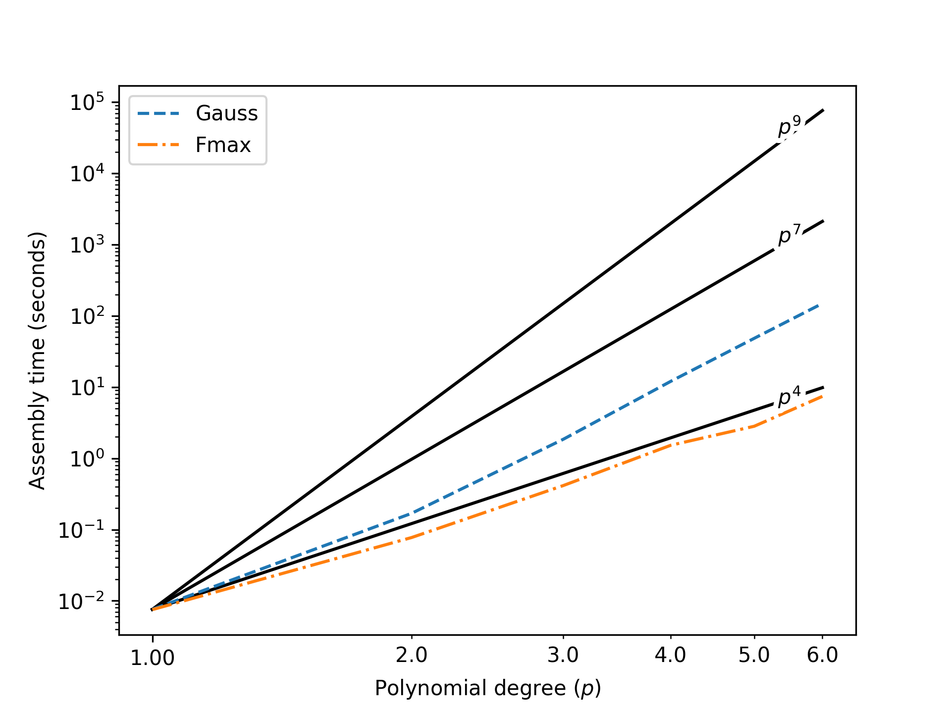
The sum factorization procedure is used for spectral elements and other higher order methods. Hiemstra et al. [42] presented results demonstrating significant improvement in formation and assembly times for single patches. These results have been reproduced in the Coreform codebase. Figure 131 shows the time spent on assembly of the mass matrix for a block as a function of the polynomial degree used to build the spline basis of maximal continuity over the block. Lines are also drawn to show the theoretically significant rates of , , and . Element-based assembly is expected to be proportional to , Gauss-based sum-factorized row assembly should be proportional to , and the reduced quadrature should be proportional to . Although we do not have benchmarked element-based assembly results here, we have included the curve for reference. The sum-factorized assembly based on a Gauss rule follows the expected rate. The sum-factorized assembly based on a quadrature rule derived from function maxima that results in ( is the parametric dimension) points per elements also exhibits the expected rate. As the polynomial degree increases, the assembly times become prohibitive. The reduced quadrature rule results in assembly times that are between one and two orders of magnitude less than the Gauss-based sum-factorized assembly which in turn is several orders of magnitude faster than the projected times for element based assembly.
Figure 131: Assembly times for a spline block with respect to the polynomial degree. Assembly times for a Gauss rule and a reduced rule derived from function maxima are shown.
13.9.5 Prospects for applying sum-factorization in practical trimmed analysis
The results of the previous section demonstrate the overwhelming advantage of sum-factorization in the situation of global tensor-product structure and high polynomial degree. However, two important questions remain: (1) how relevant are higher polynomial degrees to engineering structural analysis? And (2) to what extent can sum-factorization be exploited on trimmed patches?
For the first question, we estimate that many practitioners would find a basis polynomial degree of appealing for its ability to exactly reproduce basic beam-bending solutions, with the higher continuity permitted by isogeometric spline spaces relieving many of the robustness issues that have traditionally prevented widespread adoption of classical high-order finite elements. However, exceeding this degree would likely provide little-to-no benefit in many problems, due to several factors: (1) many practical problems have exact solutions with low regularity, to which high-order error estimates are not applicable, (2) most widely-used time integration schemes are limited to second-order accuracy, which would become the dominant source of error even in problems with smooth exact solutions, and (3) many applied problems have large inherent modeling errors, beyond which there is no benefit to further resolving the numerical approximation. For these reasons, we focus our discussion on the cases of cubic and lower degree, where constant factors may potentially outweigh algorithmic complexity advantages.
For the second question, the answer depends heavily on the type of geometries under consideration. For problems where the physical domain encloses large interior blocks with tensor-product structure, there is almost certainly a large potential advantage to applying sum-factorization on those blocks. However, many of the target problems for trimmed analysis involve intricate geometric features that are difficult to discretize by other means, and, at practical resolutions, there may be relatively few large tensor-product blocks of elements available to accelerate with sum-factorization. There are nonetheless often a significant number of individual untrimmed elements, which themselves have a tensor-product structure to exploit. The use of sum-factorization on individual elements offers a theoretical asymptotic complexity advantage over a standard quadrature loop, but less-so than the patch-level version discussed above. Thus, its usefulness for hinges on empirical testing of the constant factors affecting actual wall-clock time.
Standard quadrature
Sum-factorization
Table 14: Wall-clock time (in seconds) for tangent-matrix assembly in a heat-conduction problem, using standard and element-level sum-factorized assembly with full Gaussian quadrature.
Standard quadrature
Sum-factorization
Table 15: Analogous results to those of table 14, but using integration points per element for all , to estimate assembly cost with function-maxima quadrature.
As mentioned above, there may still be situation-specific ways to leverage sum-factorization on trimmed domains: when multiple interior elements can be grouped together into tensor-product patches or if enough of the envelope domain’s volume is occupied by untrimmed cells to make it profitable to simply integrate over the full envelope domain with sum-factorization while masking contributions from trimmed or exterior cells. However, the prevalence of these situations in target applications must be assessed critically and weighed against the code complexity entailed in automatically detecting them and following alternate code paths when appropriate.