10 Trimming
10.1 Trimmed U-splines
A trimmed U-spline is composed of a parametric atlas and associated U-spline basis and two related structures: the skin atlas that defines the boundary of the trimmed U-spline and trimmed atlas that represents the interior of the trimmed U-spline, which we summarize in figure 109. Both the skin atlas and the trimmed atlas are atlases for submanifolds of the original parametric atlas. We discuss each of these in turn.
10.1.1 Embedded Atlas
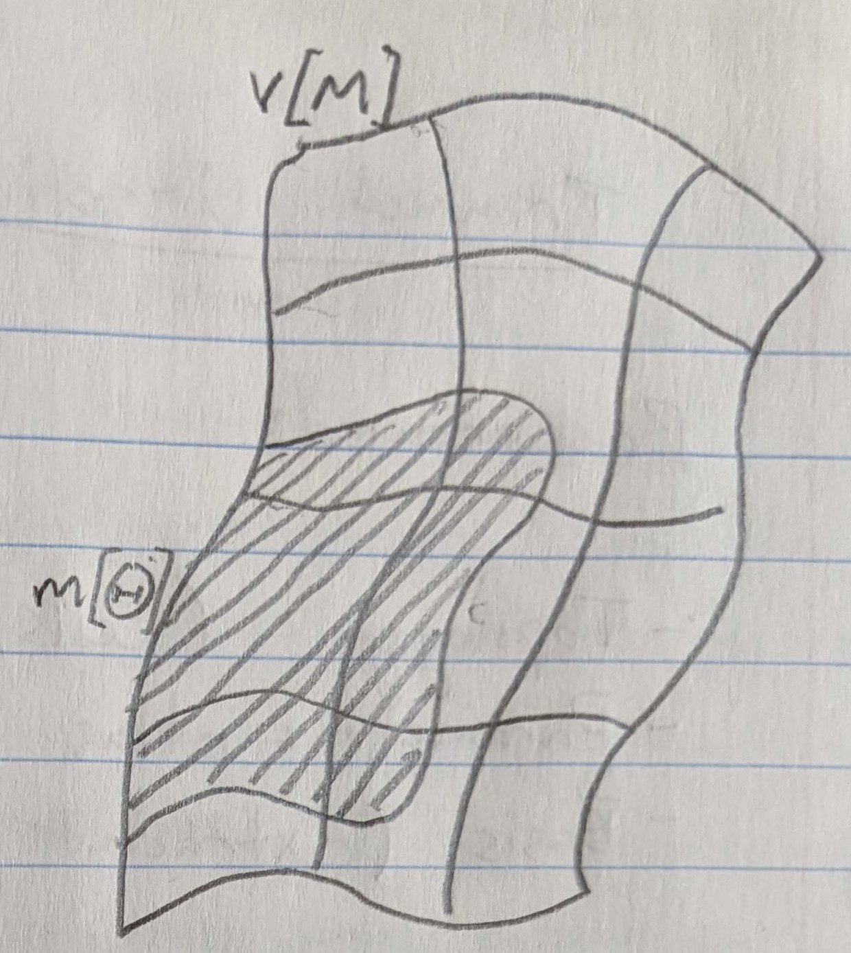
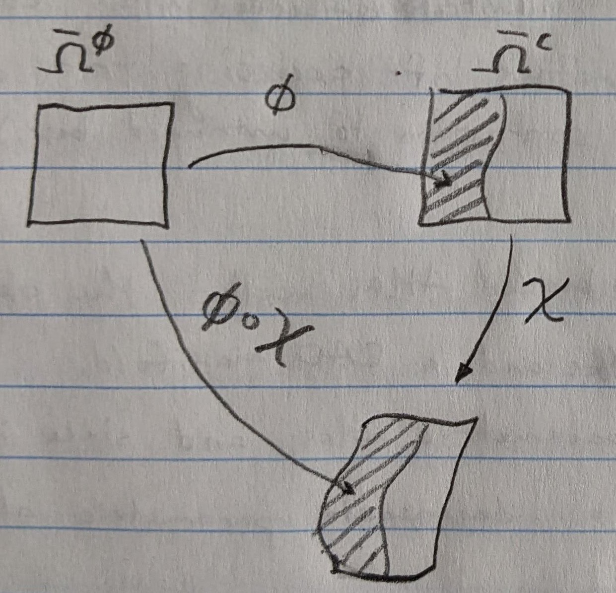
An Embedded Atlas is a collection of embedded charts, where an embedded chart is a tuple of a cell from the parametric atlas , and a chart from some parent domain to the parent domain of the cell . These charts are typically specified as a box or simplicial polynomial basis and a set of coefficients. An example of an embedded atlas is shown in the context of a parametric atlas in figure 110a. If there is a physical atlas associated with , as shown in figure 110b, composition of the charts from and can produce another physical atlas , which we term the physical embedded atlas. This composition is depicted in figure 110c.
The combined topology of the embedded charts including any coincidences of adjacent charts in defines a mesh . This mesh combined with the coordinate systems associated with each of the embedded charts forms a parametric atlas . We represent trimmed U-splines as two embedded atlases: the skin atlas and the trimmed atlas.
10.1.2 Skin Atlas
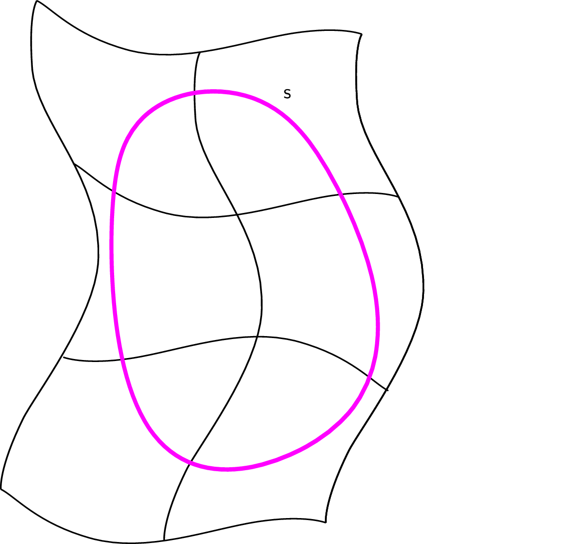
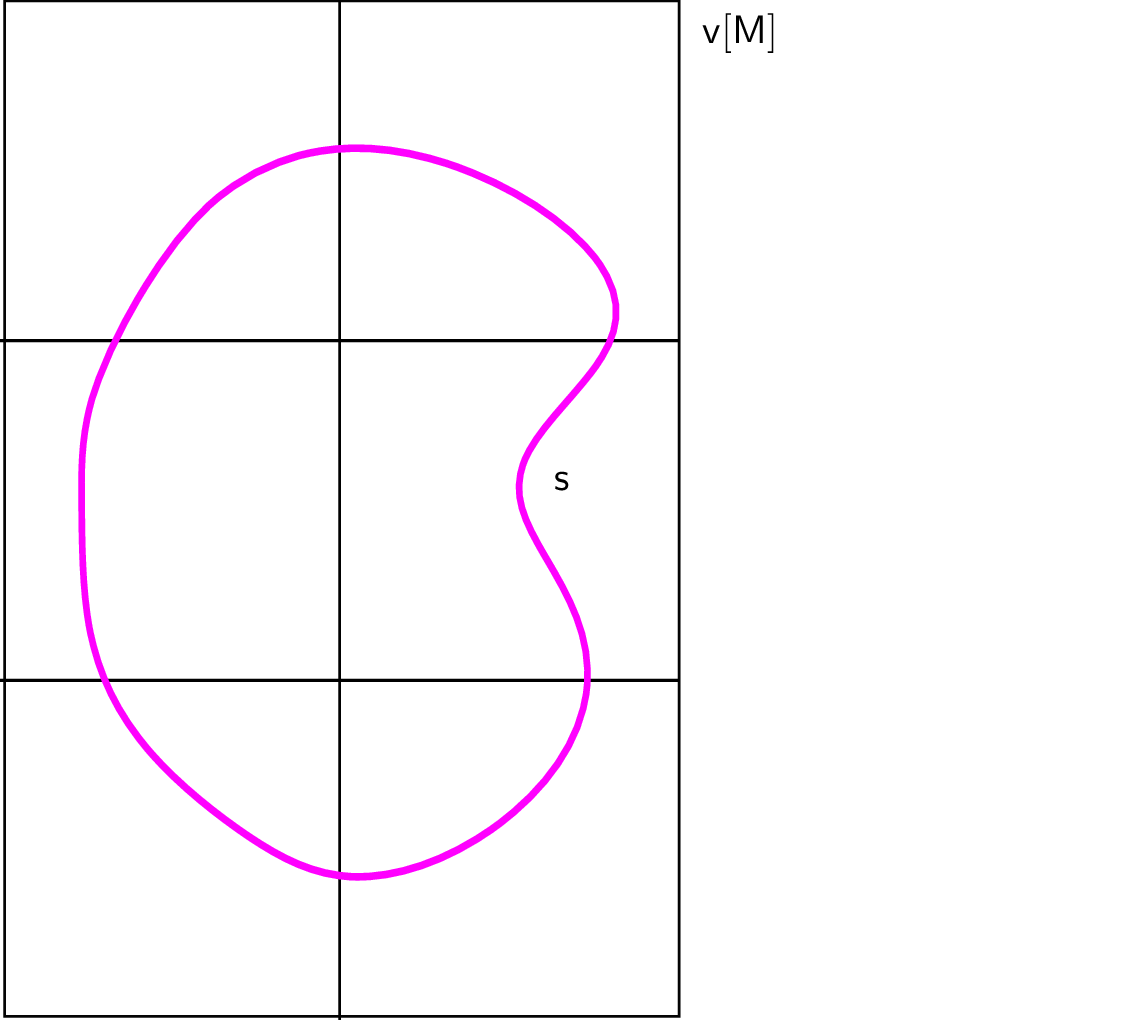
The skin atlas, , is defined by a physical atlas, , and a surface in physical space known as the trimming surface, . Each chart in the skin atlas, , is constructed so that the composition of the skin chart with the associated physical chart, produces a surface that approximates the trimming surface in some sense: where . This induces an approximate representation of the whole trimming surface in the physical embedded atlas as a composition of atlases: . We will discuss approximation metrics and procedures in a later section.
10.1.3 Trimmed Atlas
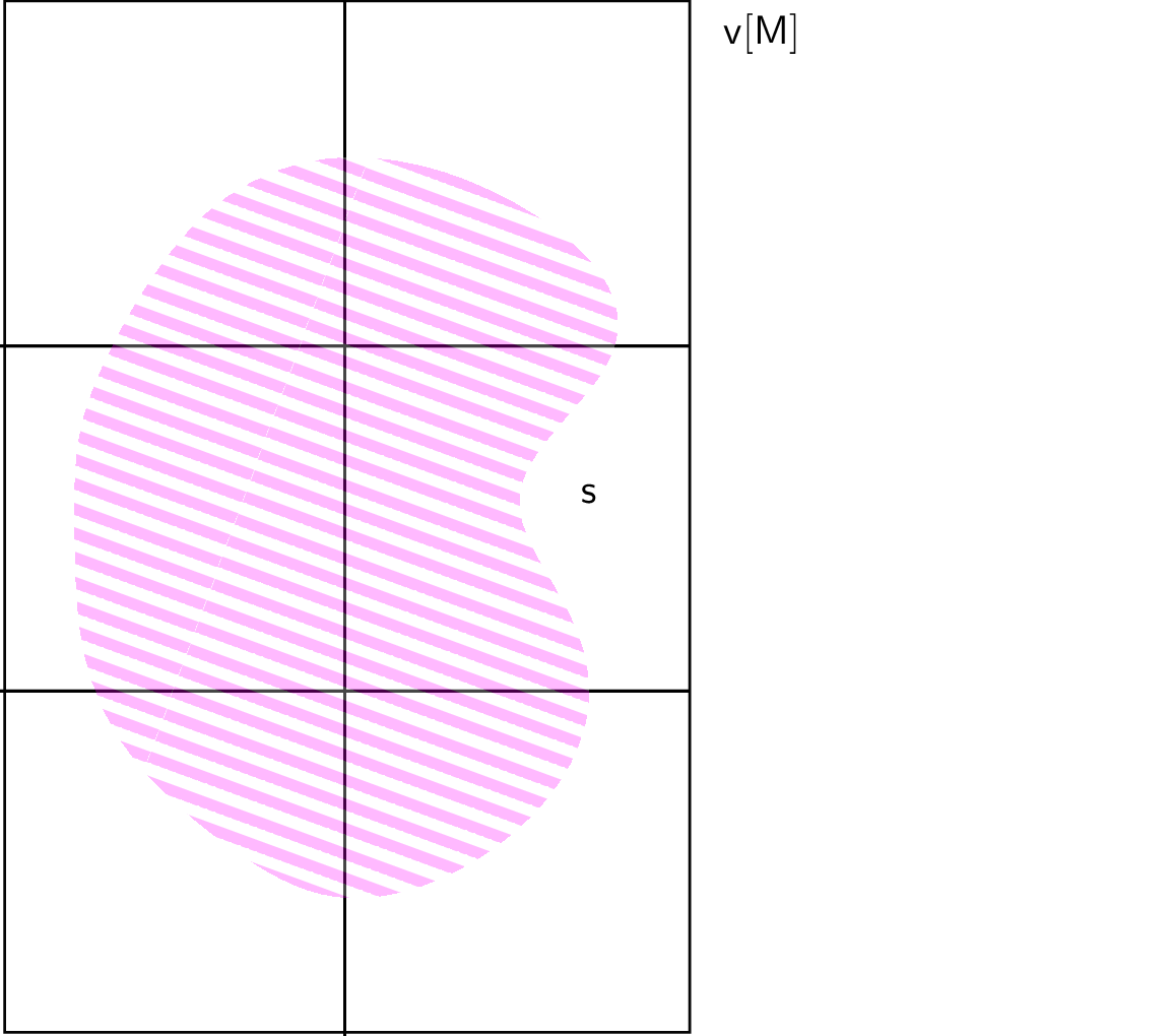
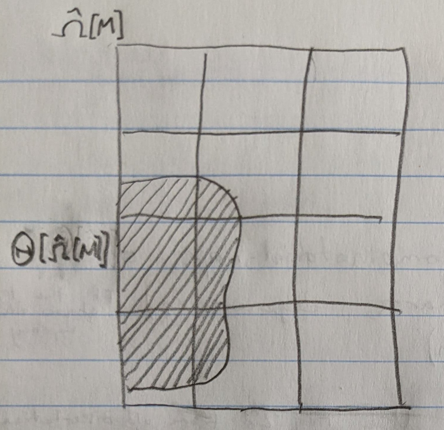
The trimmed atlas, , like the skin atlas, is defined by a physical atlas, , and trimming surface, . We require that the boundary of the charts of the trimmed atlas that intersect boundaries of the charts of the parametric atlas match the boundary of charts in the adjacent chart of the parametric atlas. This equivalence only exists under an application of the appropriate transition map of the parametric atlas. As with the skin atlas, equivalence can occur in multiple ways. We will typically require the stronger exact parametric equivalence. This provides watertight connections between adjacent charts, and allows for adjacency information in the topology of the trimmed atlas.
We require that the boundary of the trimmed atlas be equivalent to the skin atlas, . With this requirement, the trimmed atlas provides the ability to perform integration over the subset of the parametric manifold that lies within the skin atlas.
10.1.4 Chart Representation
The charts of both the skin and trimmed atlases are embeddings into the parent domain of the charts of the parametric atlas. We choose to represent each chart in both the skin and trimmed atlas as mappings generated by pairing a basis defined over a simple parametric domain (produced by a tensor product of barycentric coordinates) with a set of points chosen from the domain of the chart of the parametric atlas. The most common choice of function space and domain used to represent the atlases is the set of polynomials over a unit box. Although it is possible to use B-splines or other splines to represent each chart, we typically use a simple polynomial basis for each chart of the skin and trimmed atlases. The adaptive construction of polynomial representations described in Adaptive Construction is useful for the consruction of charts that adequately capture geometric features. Depending on the algorithm it may be convenient to represent the charts in terms of Bernstein, Chebyshev, or Lagrange bases.
It is often convenient to relax the traditional requirement that each chart be bijective and instead require only that the mapping from the parent domain of the chart be surjective for a certain subdomain of the parent domain of the associated chart in the parametric atlas. Surjectivity permits the definition of a right inverse for the chart (even though the chart is not fully invertible). This permits the use of degenerate charts in the skin and trimmed atlases. This choice provides greater flexibility in the construction of charts on complicated domains. The most common examples of degenerate charts occur when a boundary feature such as an edge or a face is collapsed to a single point or a face is collapsed to an edge. When the chart is expressed in Bernstein form, these degeneracies manifest as a set of coefficients associated with functions that are nonzero on the boundary that are all equivalent.
10.1.5 Atlas Representation
Both the trimming and the trimmed atlases carry topology and the representation data for the constituent charts. Because the skin atlas is a submanifold of the trimmed atlas, we use trimmed atlas to refer to both in this section unless a distinction is necessary.
The topology of the trimmed atlas is stored in a standard format such as a combinatorial map. The chart representations are stored in polynomial form with a polynomial basis and coefficient set associated with each cell in the topology of the respective atlas. As stated previously, each chart in the trimmed atlas is chosen as a submanifold with boundary of the parent domain of a chart of the parametric atlas. This permits the charts of the trimmed atlas to be combined with any charts associated with the base parametric atlas.
With degeneracies, the orientation of the chart coordinate systems within the cells of the trimmed atlas can only be fully specified if the combinatorial map is unoriented.
10.1.6 Skin and Trimmed Atlas Construction
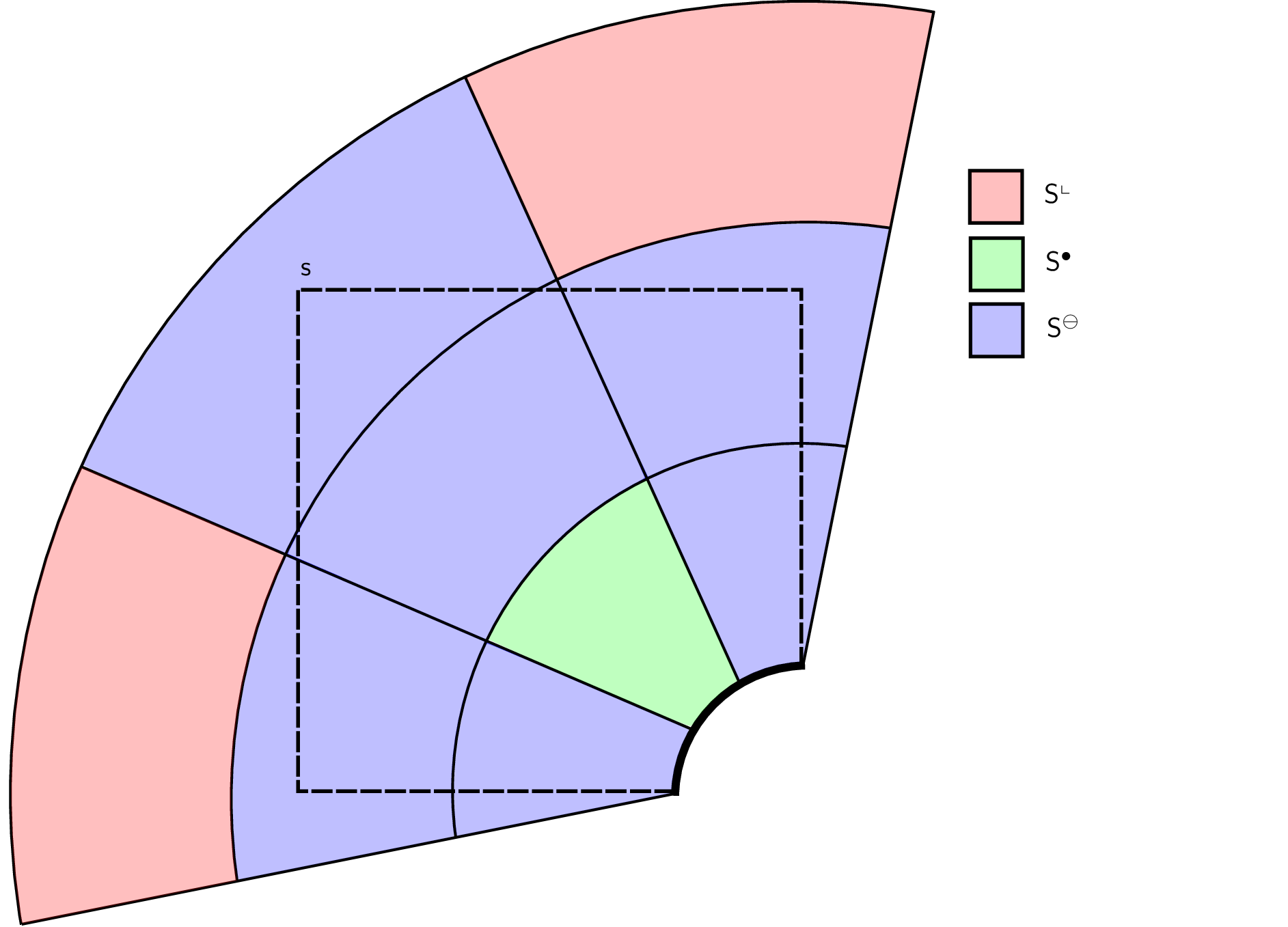
We separate the charts of the physical atlas into three sets: cut, interior, and exterior. Only the cut charts are required to construct the skin atlas. These sets of charts are illustrated graphically in figure 111.
Figure 111: The physical atlas can be separated into three sets: cut, interior, and exterior, based on how the trimming surface partitions the physical space.
At a high level, we process the portion of the trimming surface associated with each chart separately. This permits significant parallelism in the computation of the decompositions used to represent the skin atlas.
We consider a single chart and define the portion of the trimming surface that intersects this chart as . The chart inverse applied to this surface produces a surface in the parent coordinates of the chart: We construct an atlas for this submanifold by decomposing the surface . The full skin atlas is constructed by combining all of the atlases computed for all of the charts in .
In practice, in order to provide compatible connections between charts in the skin atlas, we process edges, faces, and volumes of in that order. This avoids the problem of slightly different intersections being computed on adjacent cells.
10.1.6.1 Processing Edges
A chart for each edge in is processed to determine any intersections between the trimming surface and the edge. Each edge intersection is recorded for future processing of the adjacent faces.
10.1.6.2 Processing Faces
After all edges have been processed, each face, , adjacent to an intersecting edge are processed by determining a curve, , in the parent coordinate system of the slice chart associated with the face: , , that minimizes the distance between the trimming surface and the composition of the curve with the face chart for some measure : Common choices for constructing the curve include interpolating the pullback of a set of points on the intersection of the trimming surface with the image of the face chart, ; or minimizing the integral norm approximated using a similarly computed set of points. For trimming surfaces defined in a CAD kernel, these curves are often computed by approximating the curve provided by the CAD kernel as an approximation of the chart-trimming surface intersection. Note that multiple curves may be required to capture the intersection on each face. For each volume, , with associated chart in , it will be necessary to construct the connection between adjacent curves to form loops that form connected submanifolds of . The curves representing the intersection of a face chart of the physical atlas with the trimming surface are stored so that they may be referenced in the construction of the final representation of the skin atlas.
10.1.6.3 Processing Volumes
For each volume chart, , we gather the loops formed from the curves generated in the processing of the faces adjacent to the volume. These loops are used to generate a mesh that consists only of triangles and quadrilaterals. We call this the local trimming mesh. Typically any algorithm that produces a minimal number of elements can be employed. A curve that approximates the trimming surface is generated for each edge in the trimming mesh that is not associated with a curve computed during the face chart processing phase. These curves are constructed to satisfy
Let the faces of the local trimming mesh be indicated by . The final step in the construction of the skin atlas is the construction of a chart for each face in local trimming mesh. This can be accomplished by constructing a Coons patch from the previously computed curves that bound the face. This surface is used as a starting point for the computation of the trimming chart . The trimming chart is constructed to minimize the difference between the chart and the trimming surface: Again, this is typically accomplished by interpolation or minimization of an integral approximation. The full skin atlas is constructed from the union of all trimming charts generated for each volume in . The trimmed atlas is constructed so that the slice charts on the boundary of the charts in the trimmed atlas are equivalent to the charts of the skin atlas. This is often accomplish by using Coons patches to construct appropriate charts.
10.1.6.4 Construction from ACIS Intersection Graph
The algorithm used to construct an ACISIntersectionTopology which represents an intersected volume of the background mesh with the CAD geometry (tool) is found in FnACISIntersectionTopologyCreation::buildTopology().
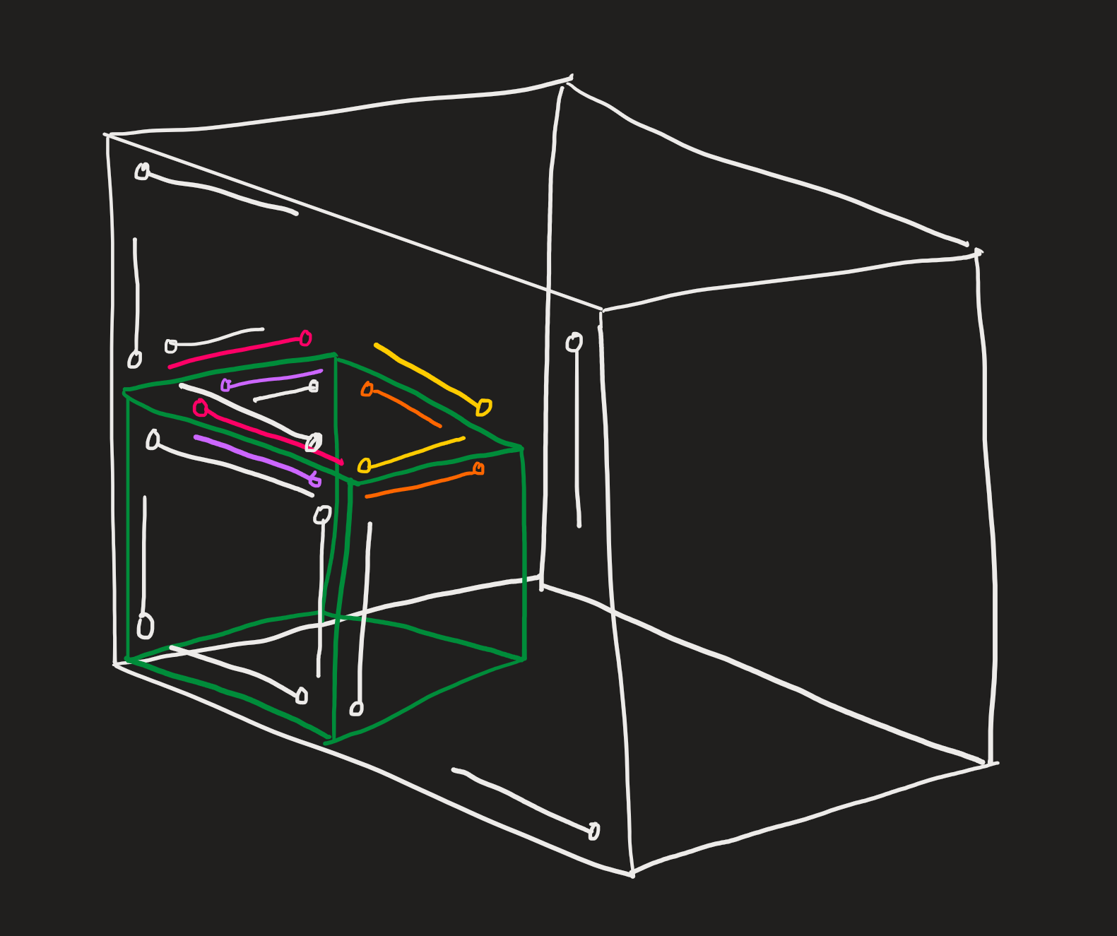
In figure 112, a volume from the background mesh (outlined in white) is being intersected with a cube (tool) in green. The cut topology darts are colored white and are shown for the front face of the volume (and several on the back face). These darts have been created during the previous step of face cutting and are copied directly into the new ACISIntersectionTopology (assigned new dart ids starting from index 0 with a mapping back to the cut topology dart id).
All the darts which have been added by face cutting or found to lie coincident with tool body faces (during face cutting) have a GraphEdge data structure associated with them. These are stored in a map during face cutting for later use in volume cutting. During the construction of the ACISIntersectionTopology, the GraphEdge data is gathered for all the darts on faces adjacent to the volume. Corresponding darts are created in the ACISIntersectionTopology for graph edges which lie on faces which extend into the interior of the volume. In figure 112, the graph darts for the top tool body face (green) are colored pink/purple and will be sewn together to create the internal face.
From these seed graph edge darts, we are able to iterate the darts around an internal face, creating new internal darts (yellow/orange) as necessary. During this process, we track the ACIS faces encountered and flood-fill to create internal darts for all the new faces encountered. The phi -1, 1, 2 and 3 connections are made at each step of the iteration around a face. The pink and yellow darts correspond to darts on the exterior of the internal faces, while the purple and orange darts are the corresponding phi 3 darts interior to those faces.
The algorithm is documented in comments in the code and there are several debugging macros that that can be enabled to dump the topology at different stages of the algorithm (define DEBUG_BUILD_TOPOLOGY) and create a .json file with the graph edges used as input (define DEBUG_GATHER_INTERNAL_GRAPH_EDGES). The best way to understand the algorithm is to step through it for a simple example like the unit test Test_FnCADTrimming::Test_SphereCuttingCubeCorner(). There is also a trim debugging guide found at https://discourse.coreform.com/t/trim-debug-guide/1809
10.1.7 The Trimmed U-spline Mesh
The resulting mesh topology of the trimmed atlas is called the trimmed U-spline mesh and denoted by . The number of U-spline basis functions defined over the trimmed mesh is denoted by and the number of elements in the trimmed mesh is denoted by .
10.2 Derivatives of Degenerate Charts
where We switch to the summation convention. In two dimensions the components of are where is the matrix that transforms the univariate Bernstein coefficients into the coefficients of the derivative. In three dimensions the components of are
For two dimensions we can flatten the transformation to a matrix for each value of : In three dimensions the three matrices are given by:
In the presence of degeneracies, the partial derivatives in the direction parallel to the degenerate edge go to zero. We can produce a derivative operator that does not go to zero by modifying .
where Another possibility is: More generally, if then we can write for linearly independent and .
We should be able to incorporate the linear terms into the operator by using Equations 2.5 and 2.6 in Sederberg’s CAGD notes:
With some manipulation we can convert to a new operator that produces coefficients for a higher degree basis in the second dimension: If we define the complement delta as then we can combine sums with different bounds: though it should be noted that if then the evaluation of the following statement should be avoided as it may result in attempting to access values that don’t exist (for ex. when ).
A similar procedure can be applied to the second component, .
Three dimensions is similar but has more terms. We will probably want to do some averaging between adjacent vertices.
If we define then a valid set is given by for linearly independent , , and . We have chosen to normalize so that the norm of , , and is 1.
The matrix forms are obtained by applying the flattening operations to the coordinate pairs:
10.3 Approximate Extracted Form
Extraction of spline basis onto an element-local basis was introduced to provide a connection between spline bases and traditional finite element assembly algorithms and data structures [14, 84]. For a cell, , in a mesh, , with an associated spline basis, , we define a local representation of the basis functions over the element as a linear combination of basis functions defined in the local coordinate system of the cell. Although it is possible to use any basis that provides appropriate properties for the problem at hand, we will restric our attention to the polynomials. Extraction was initially defined as Bézier extraction where the polynomial basis employed to represent the function locally was the Bernstein basis, but we will not restrict ourselves to a specific polynomial basis. Different bases may provide different advantages and so we will initially represent the extraction in terms of an unspecified polynomial basis with elements . Each function on the cell can be represented as where is the number of polynomial functions in the chosen basis. The standard extraction approach assumes that both and can be expressed using the same coordinate system over the cell, , and so for any piecewise polynomial (spline) basis, a local polynomial basis can be used to represent the elements of the basis over the cell. The extracted form of a spline basis provides important flexibility in the assembly and representation of spline-based simulation solutions.
In order to leverage the extraction concept in a trimmed setting, the construction of extraction operators must be modified. We wish to define extraction of the global onto a basis defined over the parent coordinates of the charts of the trimmed atlas as this is the most natural parameterization of the interior of part.
The trimmed atlas represents a decomposition of the base mesh, , used to define the spline basis. We will use to represent cells from the trimmed atlas and to represent cells from the base mesh. Each cell in the trimmed atlas has its image in the one cell of the base mesh. The set of cells in the trimmed atlas associated with a cell, , in the base mesh is represented by Each cell, , is associated with a chart
Given a global function, , in a form that permits evaluation in the local coordinates of the cell, , we wish to construct an approximate extraction that satisfies If we use to represent the coefficients that approximate generated by the adaptive computation of a polynomial representation in Chebyshev form described in Construction of Polynomial Forms then can be approximated as: where is the number of unique coefficients in . With this definition, the entries of the approximate extraction operator over , are given by The operator represents the transformation from Chebyshev coefficients to the basis .
Although the extraction operator defined in this fashion is no longer exact, it is possible to compute a sufficiently accurate approximation that provides an explicit representation of the basis functions defined over the base mesh on the cells of the trimmed atlas.
10.3.1 Extracted Tessellations
It is also useful to derive conforming tessellations from the charts of the trimmed atlas. This is most effectively accomplished by successive tessellation of the charts associated with edges, faces, then volumes (if required). By construction, the charts of the faces conform to the edge charts and similarly the volume charts conform to the face charts. The tessellations on different features may require different resolutions; adjacent tessellations that don’t match can be made to match by removing the simplices on the junction and generating a tessellation that matches both sides.
Various strategies can be employed to generate the tessellation points. It is often convenient to use a set of points derived from the basis used to represent the chart such as the Chebyshev points of appropriate degree as the base of the tessellation.
For many applications it is beneficial to construct an approximate extraction in terms of the linear basis over a tessellation. This approximation can be constructed by sampling at the parent points used to define the tessellation or by generating a projection of the spline basis onto the tessellation. An adapted form of Bézier projection can be used to generate the tessellation extraction in an efficient manner.