3 Splines
3.1 The Bézier Mesh
A polyhedral mesh topology,
A local parameterization on each cell in the mesh,
A Bernstein space assigned to each cell in the mesh,
A minimum level of continuity specified on each interface between cells.
In this section, the notation used throughout Coreform documentation to describe a Bézier mesh is introduced.
3.1.1 Topology
Formally, the Bézier mesh is a partition of a -dimensional manifold with box and simplex -cells, , where is the dimension of the cell. More precisely, the Bézier mesh is a finite normal CW complex. While it is typical to use the term cell to refer to open subsets in the cell complex, we abuse the term and use it to refer only to the closure of each cell.
-cell
Edge
Face
Volume
-cell
Vertex
Edge
Face
-cell
-
Vertex
Edge
-cell
-
-
Vertex
3.1.1.1 Adjacencies
It is useful to define a set of -cell adjacency operators. Given a cell and a -dimensional mesh , the set of -cells adjacent to is denoted by and denotes the number of -cells adjacent to . Chained adjacency sets are written as We define the application of the adjacency operation to a set of cells as the union of the adjacency operation applied to each element in the set.
Given a -cell , , and an adjacent -cell , the set contains all -cells which are both adjacent to the given -cell and perpendicular to the given -cell , and is defined as
3.1.1.2 Cell Types
A -cell is an interior cell if every interface adjacent to is adjacent to two elements. Otherwise, it is a boundary cell. We say that is regular if it is possible to embed the adjacent elements into a regular grid. More specifically, in a -dimensional mesh a vertex is regular if all elements in are box-type and , and a -cell is regular if all elements in are box-type and . Otherwise, it is an extraordinary cell. Note that all vertices and -cells adjacent to simplex elements are considered to be extraordinary for this work. On -dimensional meshes, an extraordinary -cell is said to be valence- if .
3.1.2 Cell Domains and Parameterization
Building splines over a Bézier mesh requires that a domain and right-handed coordinate system be specified over each cell. These coordinate systems may change from cell to cell to accommodate extraordinary cells or cells of different type, such as between box-like and simplicial cells.
Each cell is assigned a parent domain and a right-handed coordinate system or, when referencing a particular cell , and , respectively. We define . Here we use to represent the disjoint union. For box cells, is assumed to be a unit hypercube with a Cartesian coordinate system and, for simplicial cells, is taken to be the unit simplex with barycentric coordinates. The parent domain is defined in this way to simplify or standardize the implementation and evaluation of a Bernstein basis.
Many situations require the use of different parametric lengths in different directions. The canonical example is nonuniform B-splines; the knot vector that defines the basis possesses intervals of varying length. Although we do not use a knot vector in the definition of U-splines, we do require the flexibility of nonuniform parametric cell lengths. Each cell is also assigned a parametric domain and a right-handed coordinate system or, when referencing a particular cell , and , respectively. We define . The parametric domain of a box cell is assumed to be a hyperrectangle with Cartesian coordinates. The parametric domain of a simplicial cell will be the convex hull described by the simplex whose edges have been assigned arbitrary lengths but which are usually set to be equal to the parametric size of adjacent box cells. Barycentric coordinates are again assumed for the simplicial parametric domain. Although not discussed further in this work, the relative parametric sizes of adjacent cells must be chosen carefully so as to admit a well-defined smooth spline basis [18].
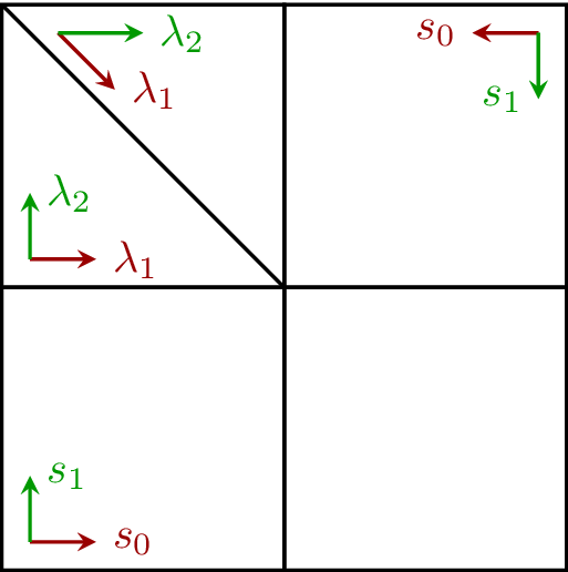
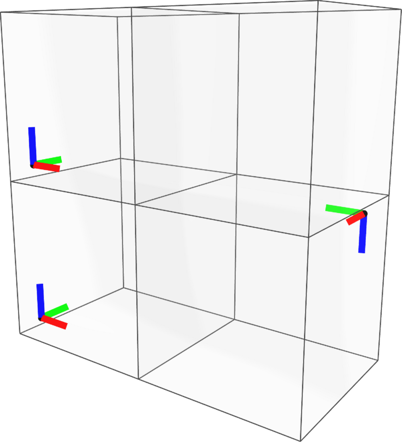
In two dimensions, we will often refer to the parametric coordinate as on a quadrilateral face and on a triangular face, as shown in figure 5a. In three dimensions, we will refer to the parametric coordinate as on a hexahedral volume, as shown in figure 5b. The operator returns the set of coordinates (or coordinate indices) in the element local coordinate system that are normal to the interface and the operator returns the set of coordinates on element that are parallel to an adjacent -cell . Similarly, returns the set of coordinates in submesh domain that are parallel to .
If required, the orientation of a cell’s parametric coordinate system will be specified by a small axis located at the origin of the coordinate system. If the small axis is omitted, a cell on a two-dimensional mesh is assumed to be oriented with the page, with the origin of the parametric coordinate system at the bottom-left corner (see figure 5a). Note that on triangles, typically only the barycentric axes associated with and are shown, since . On volumetric meshes, as shown in figure 5b, a similar small axis may be used to specify the orientation of the parameterization. The parametric coordinate systems on a volumetric Bézier mesh can be rotated relative to each other as shown on the bottom two cells in figure 5b.
For every cell , we assume there exists a linear transformation between the parent and parametric domains wherein the parametric domain can be described in terms of the parent coordinates . We denote this linear mapping by where . Note that for box cells is a simple scaling, i.e., the matrix is diagonal.
Figure 5: Examples of parametric coordinate systems specified on quadrilaterals and triangles in two dimensions (left) and on hexahedra in three dimensions (right) using small axes.
3.1.3 Cell Space and Degree
A box or simplicial Bernstein space is assigned to each cell and is denoted by . We denote the total degree of polynomial completeness of the Bernstein space on by .
The following derived quantities will be used extensively in the description of the U-spline algorithm. Let denote the degree on a -cell in the direction perpendicular to the adjacent interface and denote the degree on a -cell in the direction parallel to the adjacent edge Let denote the -dimensional tuple containing the degrees on in the directions parallel to the cell . We can then define the useful operators , , , and as Note that in a simplex cell, these derived quantities are equal to the base degree.
To measure the the minimum or maximum degree in a direction parallel to an interface and perpendicular to a -cell adjacent to the interface , we define and as
3.1.4 Interface Continuity
Given a -dimensional mesh , each interface is assigned a required minimum continuity . We denote the continuity assigned to an interface by . Note that for certain mesh configurations, the U-spline basis may be smoother than the specified conditions on the interfaces. We say that an interface has reduced continuity with respect to an adjacent -cell if where is the degree on a -cell in the direction perpendicular to the adjacent interface . We say that an interface is creased if it has been assigned or continuity, and that a -cell is creased if all adjacent interfaces are creased. The operator returns the maximum continuity of all the interfaces that are both adjacent to the given -cell and perpendicular to the given -cell , and is defined as where
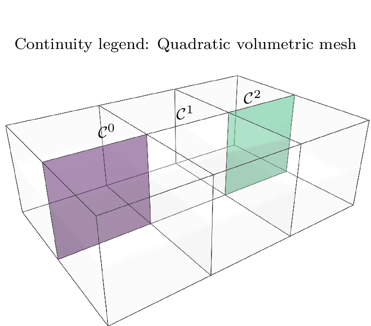
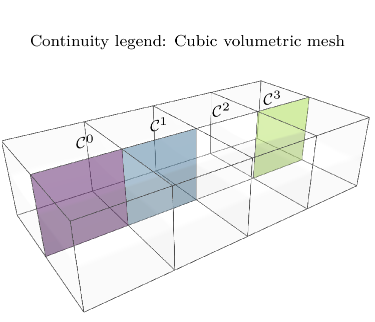
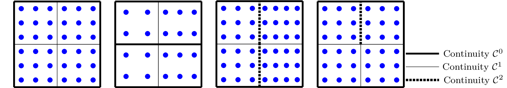
The continuity of interfaces on two-dimensional figures will be indicated by an accompanying legend or a description in the caption. The continuity of interfaces on volumetric meshes will be indicated by the description in the caption and will follow the pattern indicated in figure 6. The most common continuity in the mesh and boundary interfaces are often left colorless for greater clarity.
Figure 6: The continuity of interfaces on volumetric Bézier meshes are indicated by the color of a semi-transparent surface drawn on the interface.
3.1.4.1 Supersmooth Interfaces
When setting the smoothness of an interface we normally require that and say that is maximally smooth if
Additional options are possible with U-splines. We say an interface is supersmooth if
for some element adjacent to . If, additionally
then the supersmooth interface is in fact . Note that a supersmooth interface is a generalization of the concept of T-junctions [88].
We do not explore this concept further but rather restrict supersmoothness to the simple case where, given two elements and that share interface , we allow and require that and .
Figure 7 shows several examples of supersmooth interfaces. On the left, an example of a two-dimensional Bézier mesh with maximally smooth interfaces (equation ) is shown. The two meshes shown in the center have supersmooth interfaces with differing perpendicular degree (equation ). On the right, a supersmooth interface in a configuration which is equivalent to a T-junction (equation ) is shown.
3.2 Bernstein Representations
We now turn our attention to how spline functions are defined over a Bézier mesh. As discussed previously, classical spline technologies, such as NURBS and T-splines, rely on a certain level of global structure to define basis functions. In the case of NURBS, all cells in one direction must use the same polynomial degree and higher-dimensional splines are constructed by global tensor products of univariate NURBS. T-splines also require the specification of global polynomial degree and, while T-splines require less global structure than NURBS, each T-spline basis function is constructed on a local tensor product region. For T-splines, it can be difficult to infer the properties of the underlying spline space by examining the associated T-mesh.
A key practical and conceptual development in the field of IGA was the advent of Bézier extraction as an analysis technology. Bézier extraction allows global spline functions to be evaluated locally on a Bézier cell [14, 84]. More generally, Bézier extraction is a method of providing a Bernstein representation of spline functions while maintaining the connection to global spline representation. Bernstein representations are central to representing U-splines, and this section serves to present the necessary notation that will be used throughout the rest of this manual.
3.2.1 Indexing
The th Bernstein polynomial on a -cell in the mesh forms a unique index, denoted by or , that specifies both and the local Bernstein function index . For simplicity, and when the meaning is unambiguous, we will often just use to denote both the function index and cell. The set of all indices for all Bernstein polynomials defined over all cells in is denoted by and is used to represent the indices for . We denote the number of indices in any index set by . The cell associated with a given index is denoted by and the set of cells associated with an index set is written as We will often denote a set of index sets by .
Figure 8 shows an example of indices on two-dimensional cells. The positioning and quantity of indices indicates the polynomial degree of the Bernstein functions on each cell in each parametric direction. For example, the quadrilateral cell in figure 8 is quadratic in and cubic in . On triangular cells, we follow the convention of listing only indices and since on a two-dimensional simplicial Bernstein polynomial, one of the indices is fixed by the choice of polynomial degree and the other two indices: , . In figures where the specific index is either apparent from context or not required, we represent indices as small circles or spheres as shown in figure 8, figure 9. Note that we draw these circles inset from the boundary of the cell to avoid confusion between functions on adjacent cells.
Figure 8: The Bernstein indices (on the left) and corresponding circles (on the right) for a two-dimensional mesh with a quadrilateral and triangular cell, with degrees and , respectively.
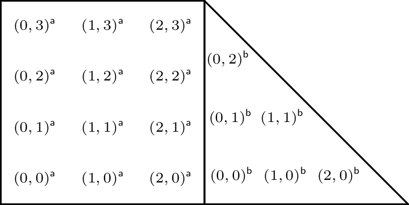
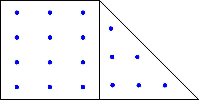
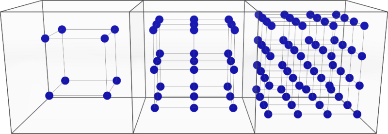
Figure 9: We depict Bernstein indices in volumetric cells as small spheres, the positioning and quantity of which indicate the polynomial degree of the Bernstein functions on each cell in each parametric direction. The cells from left to right have degrees , respectively.
3.2.2 Bernstein Form
We say that a piecewise function can be written in Bernstein form on the mesh if it may be expressed as a linear combination of the Bernstein polynomials on each -cell in the mesh. In other words, given a set of Bernstein coefficients the Bernstein form of is We will often use the Bernstein coefficients of and the function interchangeably.
The index set of , or equivalently, , is by definition since the domain of is . Functions that are nonzero on only a portion of the Bézier mesh will typically have a large number of zero coefficients and so we adopt a sparse representation that contains only the indices that correspond to nonzero coefficients. The indices associated with the nonzero Bernstein coefficients in or is denoted by
The nonzero support of , denoted by or , is the parametric domain over which the function is nonzero
Given a function in Bernstein form and an index set , we define the restriction of , denoted by or, equivalently, , to be the function having the same Bernstein coefficient values as for all indices in and zero for all indices not in .
3.2.3 The Trace Mapping Matrix
Assume that we are given an element , with associated parametric domain , and an adjacent (lower-dimensional) interface , with parametric domain , and a map , and Bernstein bases and satisfying (all functions from the element basis can be represented as linear combinations of interface basis functions). Then, the components of the trace mapping matrix are where is dual to in the sense that [50].
We use to indicate the th directional derivative of the function with respect to the direction perpendicular to the interface . The components of the trace derivative mapping matrix are
For a given the set of indices on that correspond to the nonzero coefficients on the th row of is denoted and is defined as Note that, in practice, there are efficient approaches for determining the indices of the nonzero coefficients of the trace mapping matrix without computing the matrix terms via integration.
3.3 Continuity Constraints
As mentioned in The Bézier Mesh, a Bézier mesh has a prescribed minimum continuity assigned to each interface . That is, a piecewise function defined over should have at least continuous derivatives across . Given a function in Bernstein form, we may state a continuity constraint in terms of the function’s Bernstein coefficients, . We denote a set of continuity constraint coefficients as . Then, we may write a homogeneous continuity constraint on a piecewise function in Bernstein form as
An abstract approach to assembling the constraint sets is presented here, which may be applied to determine the constraint equations for meshes of any dimension.
3.3.1 Constraint Sets
The set of continuity constraints associated with an interface is denoted by and the set of all continuity constraints defined over is denoted by
Given a -dimensional cell , , the associated set of continuity constraints is the union of all constraint systems associated with interfaces satisfying :
Given an index set and a continuity constraint, , the restriction of the constraint to the index set is the constraint that results from keeping only the coefficients associated with indices in the index set. It is denoted by . Given an index set and a set of continuity constraints , we denote the restricted set of continuity constraints by In other words, any constraints that are empty after the restriction to the index set has occurred are removed.
3.3.2 Constraint Matrices
Given a set of continuity constraints , an index set , and a function that assigns a unique integer to every index in , we can construct a matrix , called a (restricted) constraint matrix. For simplicity, the constraint matrix associated with a -cell is denoted by and the constraint matrix for the entire Bézier mesh is denoted by .
3.3.3 Constraint Construction
We consider constructing constraints on the interface between two elements and on a -dimensional Bézier mesh, where . Assume we have two functions defined in Bernstein form: defined over as and defined over as We also require the maps from the shared interface to and : and .
If the functions and satisfy
for any then we say that they are value continuous or . This pointwise constraint over the interface can be converted to a constraint on the coefficients that define the two function through the use of the trace mapping matrix defined previously.
We choose a basis defined on the interface that is sufficient to generate the trace mapping matrices for both and : and . Equipped with these matrices, the value constraint given in equation is equivalent to for all indices associated with the basis selected for the interface. It is often convenient to express constraints in homogeneous form: Continuity constraints associated with the th derivative can be constructed by using the matrices and .
Other work has been done that allows for higher-order continuity constraints for simplex cells to be stated similarly [73]. Thus, the continuity constraint equations are
3.4 Splines and the Nullspace Problem
Given we can form the corresponding vector nullspace problem: Determine the nullspace where
The rank-nullity theorem tells us that the dimension of the nullspace is .
3.4.1 Basis Vectors
As with any vector space, any vector in can be represented as a linear combination of the members of a linearly independent set of vectors. The th such vector is called a basis vector, denoted by , and the set of basis vectors, denoted by , form a basis for the nullspace. Of particular importance is determining a sparse positive basis for . This means that we seek to find a set of basis vectors where the set of Bernstein coefficients that define the basis vector has a small number of positive nonzero coefficients (and no negative coefficients). For the cases considered here, the sparsest positive basis is sufficient. In cases where choices must be made, we choose bases in which a certain notion of connectedness is maintained. We do not discuss this at this time. The set of indices associated with the nonzero coefficients of a basis vector is sufficiently important that we introduce the symbol to represent these sets. We also define the set of index sets associated with the basis vectors
3.4.2 Basis Functions
Since the Bernstein coefficients that compose each basis vector correspond to a set of Bernstein basis functions,we can also formulate an equivalent operator nullspace problem. In this case, the commonly used terminology changes slightly: Given the Bernstein space , the constraint space , and the linear constraint operator , determine the linear subspace of , called the kernel or nullspace of and denoted by , where
In this case, there is a set of functions, denoted by , that span the null space . The th such function is called a basis function, denoted by .
3.4.3 Spline Form
Due to the equivalence between equation , equation , the basis functions in not only define directly as but are also written in terms of the basis vectors in as
where .
Importantly, since each satisfies the continuity constraints on , it is immediately obvious that is not only a function in Bernstein form but also a spline—
3.4.4 Extracted Form
For convenience, we often arrange the Bernstein and U-spline basis functions that are nonzero over a -cell into vectors, denoted by and , respectively. We can then arrange the Bernstein basis vector coefficients on for each U-spline basis function into corresponding rows in a matrix , called a cell or element extraction matrix. We then have the extracted form of the U-spline basis:
In this case, we call the Bernstein basis vector coefficients extraction coefficients. Note that at times it is convenient to combine the cell extraction matrices into a global extraction matrix . Representing U-spline basis functions in extracted form is a powerful and convenient abstraction when generalizing finite element frameworks to accommodate smooth spline bases like U-splines. In particular, it is the preferred and simplest representation for smooth splines when the underlying algorithms used to generate the spline basis are not the primary concern.