14 The Flex Representation Method
14.1 Flex Modeling and Spectrum
During the creation of a trimmed U-spline, the modeler or analyst can choose the optimal level of effort to generate the physical atlas , which we will simply call the U-spline. Common considerations are the difficulty in generating the underlying mesh, the resulting properties of the trimmed U-spline basis, or the physical characteristics of the simulation problem to be solved. Since there is an inherent flexibility in how is modeled, we call the process of building flex modeling and the associated numerical models that process trimmed U-splines flex representation methods. In all cases, the approximation power of the higher-order, smooth, locally-adaptive U-spline basis underlying will continue to produce accurate solutions.
We call the set of all potential flex modeling approaches for a given problem the flex spectrum and denote it by and refer to a unique instance within the spectrum as . By convention, we use to represent the fully-featured, body-fitted approach (shown in figure 132a), to represent the partially defeatured, body-fitted approach (shown in figure 132b), and to represent a traditional fully-immersed approach where all geometric features are retained but immersed in a background mesh. These symbols represent the extrema of Positive integers are then used to communicate the ordering of instances or indexing along the interior of , with larger indices suggesting higher levels of immersion. A single flex model in the interior of will simply be denoted by .
14.2 An Illustrative Example
In the example shown in figures 132, 133, 134, and 135, an experienced analyst has devised five potential simulations within . In figure 132, the features that the analyst has selected for defeaturing (light highlight), immersion (medium highlight), or body-fitting (dark highlight) are shown. Note that in none of these examples is the model both defeatured (thus modifying the physical domain) and immersed. This combination is possible within the flex spectrum, but omitted here for simplicity.
: In , shown in figures 132a, 133a, and 134a, no surfaces have been selected for defeaturing or immersion. In other words, the U-spline, shown in figure 133a, is equivalent to the physical domain . For an experienced analyst, producing the mesh for , shown in figure 134a, requires approximately twelve labor hours. This estimate includes significant time spent correcting inconspicuous geometry errors in the native CAD definition that nevertheless complicate or even prevent the successful generation of a mesh.
: A more sensible approach is taken in , shown in figures 132b, 133b, and 134b, where the analyst recognizes that the CAD features shown in figure 132b will complicate the meshing process and can be safely removed, resulting in the defeatured CAD model shown in figure 133b. The mesh generation process is much simpler for than for , requiring only a few minutes of analyst time to produce, as shown in figure 134b.
: Wishing to retain the computational efficiency of , but hoping to avoid potential errors caused by CAD defeaturing, the analyst instead immerses the complex CAD features, as shown in figures 132c, 133c, and 134c. The resulting U-spline, shown in figure 133c, is similar to , shown in figure 133b, and can be meshed using a similar strategy, as shown in figure 134c, although this will not generally be the case. In fact, the U-spline mesh generation process should become more simple as the spectrum index increases and more of the model is immersed.
: In , the analyst seeks to eliminate the meshing problem entirely by immersing all but the outermost features, as shown in figures 132d, 133d, and 134d. As a result, the analyst produces the U-spline shown in figure 133d. In this case, no decomposition step is required to produce the mesh shown in figure 134d. By fitting the U-spline to major features of the physical domain, significant accuracy gains are realized in comparison to .
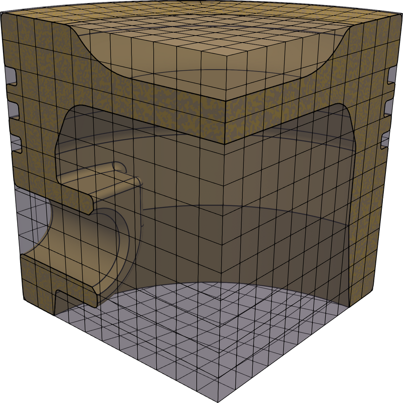
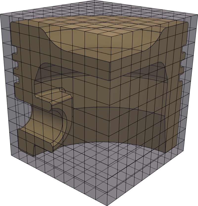
: In , all features of the CAD geometry, shown in figures 132e, 133e, and 134e, are immersed within the rectilinear U-spline, shown in figure 133e. As shown in figure 134e, this rectilinear U-spline is trivial to mesh. In this case, the analyst has in fact eliminated all manual labor associated with mesh generation. While all the previous approaches can utilize adaptivity to boost accuracy, will in most cases require local adaptivity to produce the best results.
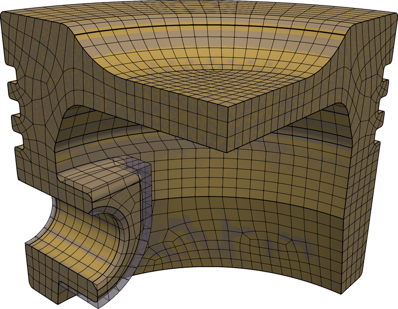
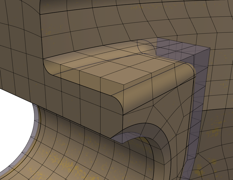
The U-spline associated with each flex model are shown in figures 135a, 135b, 135c, 135d, and 135e. We again note that both and have U-splines that are equivalent to their respective physical domains, while have at least part of the physical domain immersed within the U-spline. As expected, has the highest element count of the alternatives shown, due to the requirement that the mesh both fit all small features in the CAD model and be a conforming hexahedral mesh. A closeup of a partially-immersed CAD feature is shown in figure 136.
Figure 132: An example flex spectrum. The CAD surfaces that will be defeatured (light highlight), immersed (medium highlight), and body-fitted (dark highlight) are highlighted.
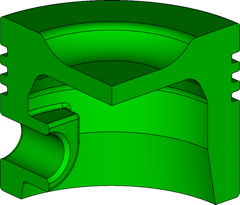
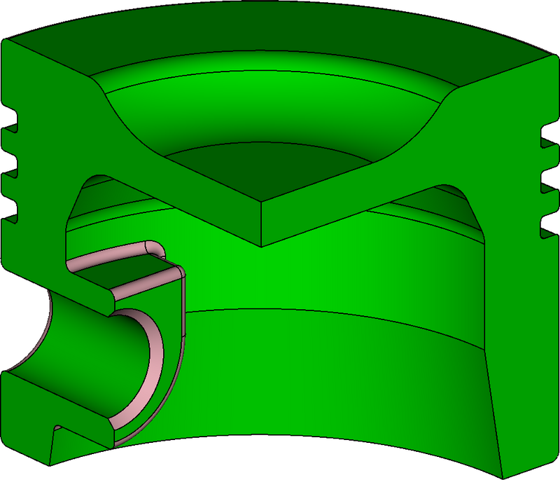
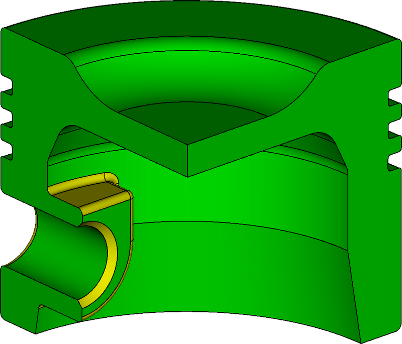
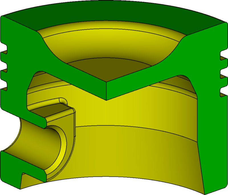
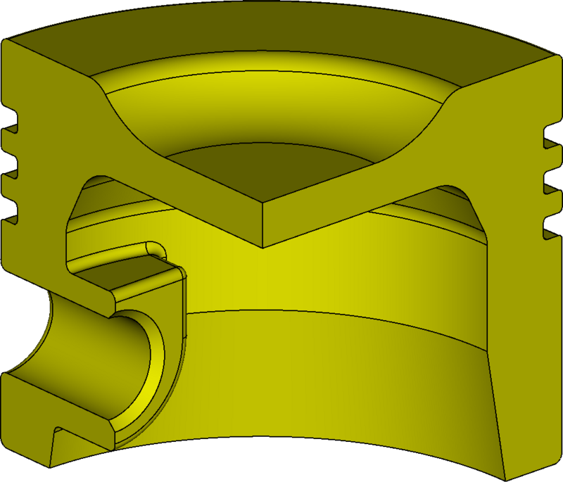
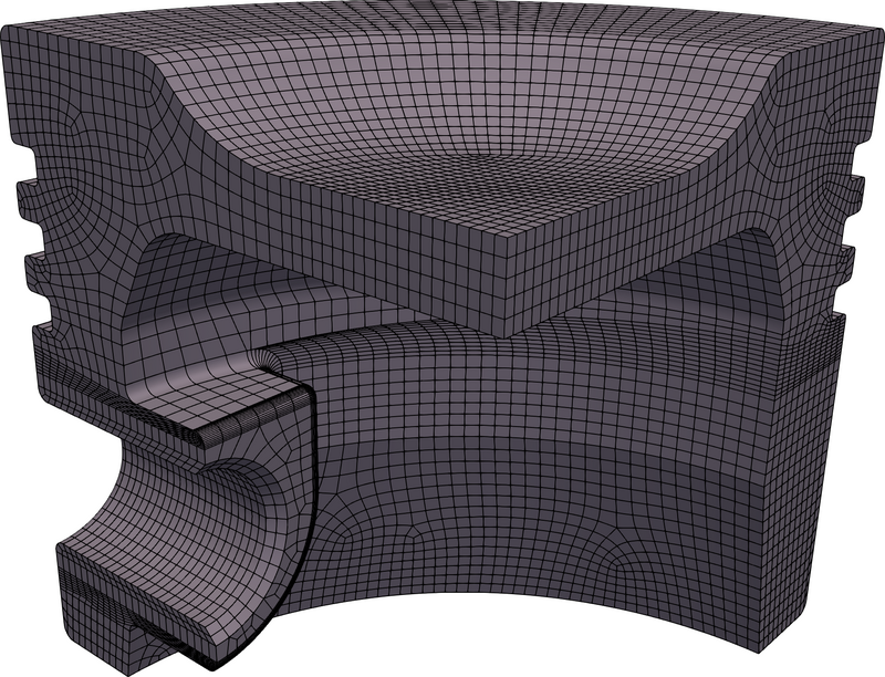
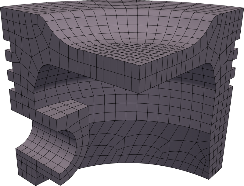
Figure 133: The CAD geometry that the U-spline will be fit to for each approach.
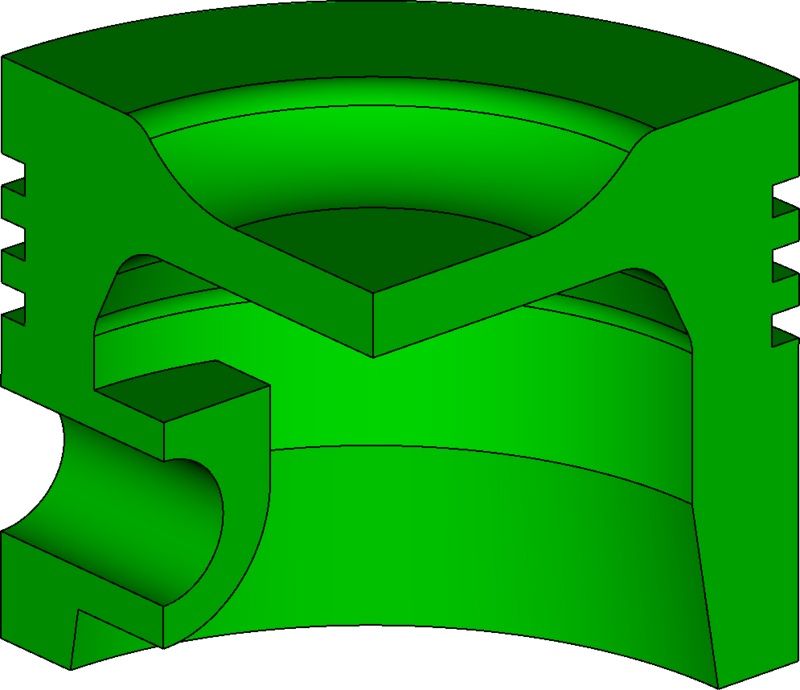
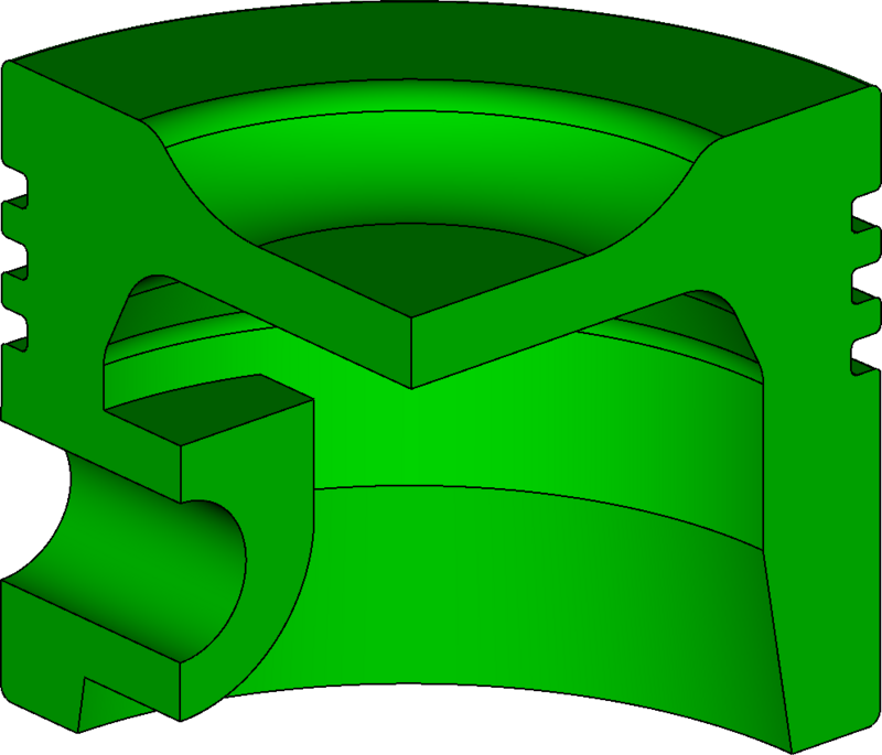
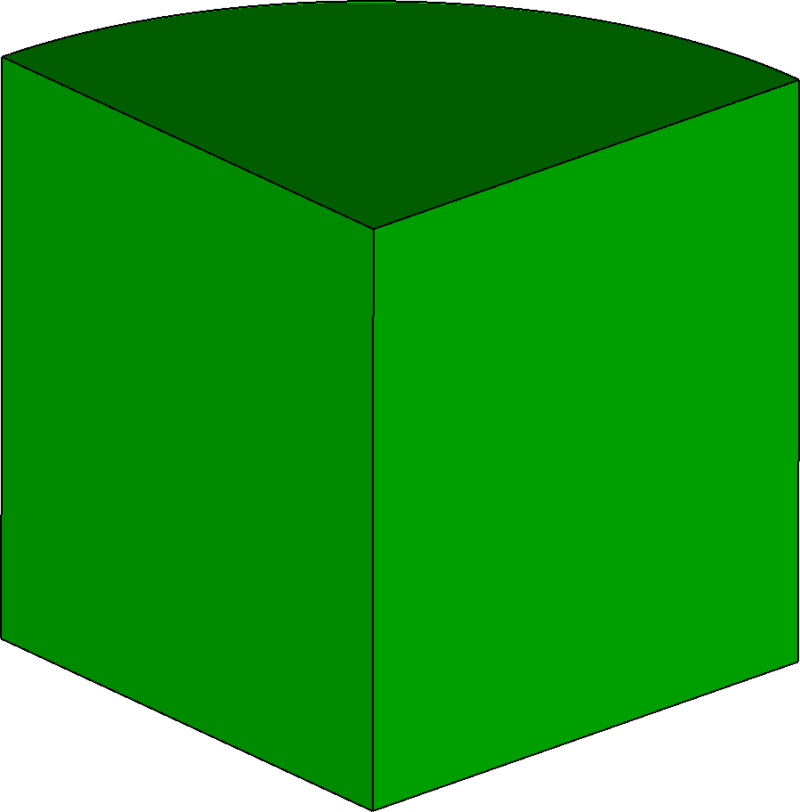
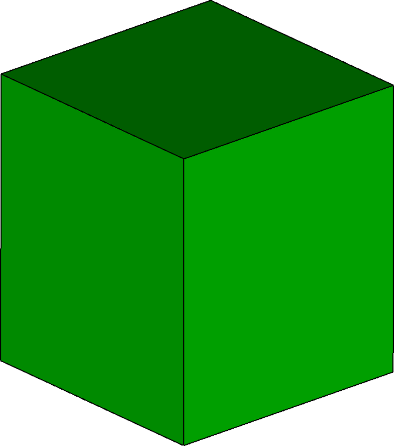
Figure 134: A comparison of the decompositions and resulting hexahedral meshes for each approach.
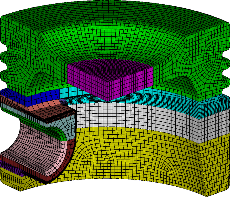
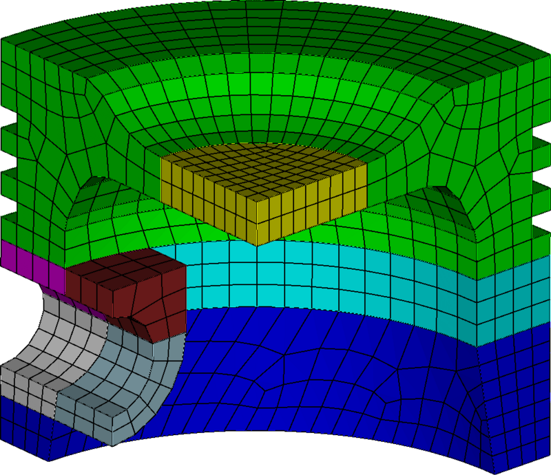
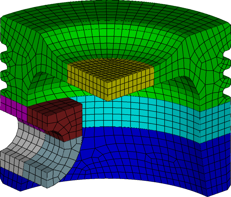

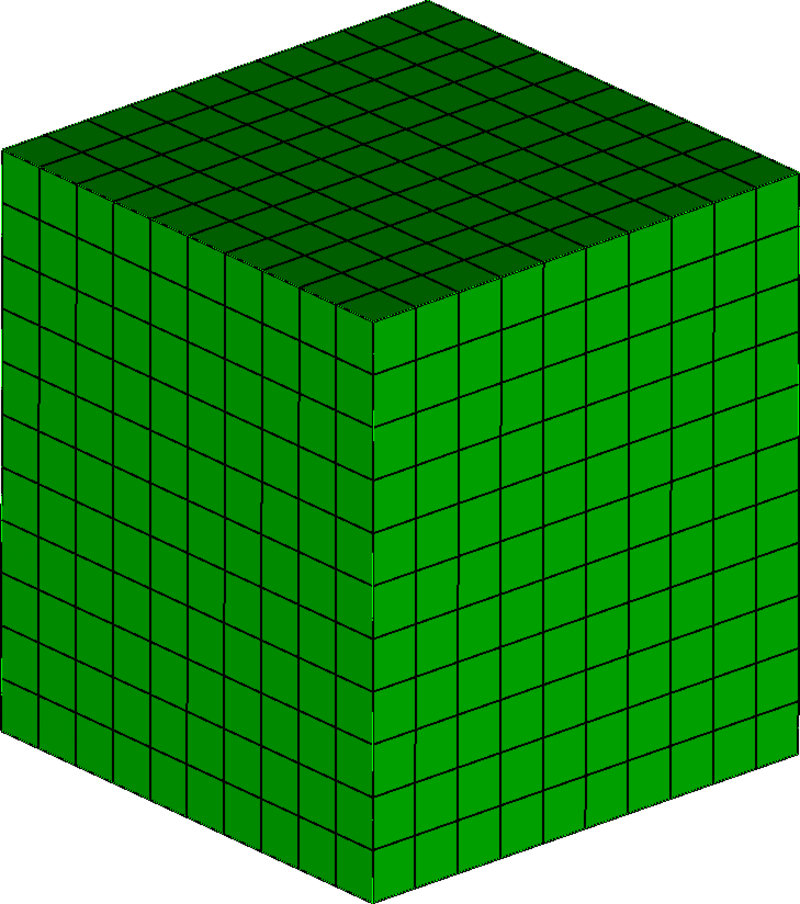
Figure 135: The U-splines for each approach. The associated physical domain, when different than the U-spline domain, is also shown.