4 U-splines: Definition
4.1 Summary
Computer aided engineering (CAE) can provide feedback regarding the expected behavior of a given part before costly fabrication is undertaken. The predominant simulation technique in current use in CAE is finite element analysis (FEA). In FEA, the simulation of a computer aided design (CAD) is typically preceded by a process known as meshing, in which a faceted approximation of the original CAD model is constructed to satisfy the requirements of the simulation pipeline. Inconsistencies in common industrial CAD representations, such as small gaps between adjacent CAD faces, must be resolved during the meshing process resulting in a final mesh approximation that is referred to as “watertight” or “analysis-suitable”.
A faceted mesh is a piecewise-defined function that satisfies continuity constraints between adjacent cells. The function, restricted to the domain of each cell, is a linear polynomial or facet. Across interfaces, or the boundary of adjacent cells, the function is -continuous. Continuity or smoothness refers to the level at which a function shares the same values on either side of an interface. If the function is discontinuous at the interface then the function can have different values at adjacent points in the cells on either side of the interface. A function is said to be value continuous if the function produces the same value at points in each cell that are adjacent across the interface. Other levels of continuity are also possible; the slope and curvature of the function can also be continuous across the interface. Higher levels of continuity require mathematical definitions in terms of derivatives. We say a function has continuity of order where ; we also say a function is -continuous. is discontinuous, is value continuous, etc.
While it is technically correct to call a faceted mesh a spline, the term spline has become synonymous with meshes of higher degree and continuity. We will often use the term smooth spline to disambiguate the term. The most recognized example of a smooth spline is the B-splines or basis splines. Originating with Cox, de Boor, and Mansfield, the basis spline functions are the minimally supported spline functions on a partitioning of an interval. The minimal, compact support of B-splines is significant for both design and simulation.
The simplicity and efficiency of prevailing smooth spline constructions, their superior approximation properties, and numerical robustness have led to the widespread industrial adoption of smooth splines as the foundation of modern CAD tools. Indeed, nonuniform rational B-splines (NURBS), a generalization of B-splines, are foundational to virtually all CAD modeling environments, where they are used primarily for non-analytic curve and surface representation.
Interestingly, the superior behavior of smooth splines, when applied to FEA has long been recognized by analysts [106]. However, most splines, other than simple splines, were viewed as too expensive or the construction too complex for general-purpose FEA. Efforts were made to improve the geometric definition in FEA through the use of subdivision surfaces [20] and NURBS in FEA [43], among others, but it was not until the introduction of the concept of isogeometric analysis (IGA) [46] that a large-scale effort to exploit the properties of splines in FEA commenced. IGA can be understood simply to be FEA with smooth splines. The potential benefits of this approach have become clear [25, 37, 63], but the watertight meshing of complex CAD geometries with smooth splines remains a significant barrier to broader adoption.
Our opinion is that a smooth spline meshing technology for industrial-scale FEA problems should be capable of smoothly and accurately representing complex CAD models, be compatible with prevailing industrial spline representations such as NURBS and T-splines, support the local modification of cell size (-refinement), degree (-refinement), and intercell continuity (-refinement), naturally generalize to higher dimensions, and provide a locally-supported, complete, positive basis for the underlying spline space that forms a partition of unity and is (locally) linearly independent. The U-spline technology satisfies all these technical objectives.
4.2 Previous work
The need for advanced smooth spline surface meshes in CAD and, in particular, animation and graphics applications, led to the development of both subdivision surfaces [68] and later T-splines [88]. A significant benefit of the T-spline construction is its compatibility with NURBS representations. Additional developments to follow on the advances of subdivision surfaces and T-splines include PHT-splines [27] and polynomial splines over T-meshes [55]. In these works, the continuity of the splines is restricted to be less than half of the polynomial degrees on adjacent cells. The importance of handling singular or extraordinary vertices smoothly has long been recognized and many approaches have been proposed [66, 76, 110].
The potential benefits of smooth unstructured spline meshes was recognized soon after the advent of FEA [5]. Despite these early efforts, the majority of finite element research was carried out on constructions and so FEA came to be associated primarily with basis functions. More recently, subdivision surfaces were applied to shells [20]. Shortly after the original introduction of IGA [46], work commenced on IGA based on T-splines [10]. This was motivated by both the unstructured nature of T-splines and the need for adaptive local refinement. The need for guarantees on analysis properties of the basis led to the introduction of analysis-suitable T-splines (ASTS) [53]. Other efforts to produce refineable splines suitable for use in FEA followed such as locally refined (LR) B-splines [28] and hierarchical B-splines and truncated hierarchical B-splines [38, 86]. Constructions based on geometric rather than parametric continuity have also been explored [40, 51].
There has also been significant work on spline constructions over unstructured meshes within the wider numerical analysis community, although many of these approaches have not been widely adopted in FEA. Classic approaches commonly employed to produce continuity greater than include Arqyris elements [5], Clough-Tocher elements [4], and Powell-Sabin splines [102, 104] among others. Significant work has been carried out on the dimension of spline spaces for both triangle [3, 52] and T-meshes [54, 55]. Meshes consisting of both squares and triangles with potentially hanging vertices, also called T-junctions, have been considered [83] although only splines of continuity were explored. The approximation power of splines over T-meshes for splines of reduced continuity greater than has been established [83]. Several types of simplex splines have been introduced to facilitate the construction of splines in unstructured settings [65]. Several adaptations of simplex splines to Powell-Sabin and other splits have been proposed to allow their use on unstructured meshes [21, 59, 105]. Additional methods combine the solution of continuity constraints together with the solution of the governing PDEs [8, 44, 82]. Splines based on both triangles [49, 67, 115] and tetrahedra [114] have been employed in IGA.
Practical constructions of mixed degree or multi-degree smooth splines are currently limited to univariate constructions and their tensor products and consequently have not seen extensive use in FEA although basic constructions are used in -adaptive methods [26]. In CAGD, univariate mixed degree or multi-degree splines have been proposed [89, 90, 108]. We should mention that multivariate multi-degree splines with higher continuity have been constructed on triangulations without a basis for the purpose of numerical analysis [44].
While B-splines, due to their tensor product structure, naturally generalize to arbitrary dimensions, it remains a challenge to generalize less structured splines to higher dimensions. Initial efforts have been made to parameterize an irregular volume with a collection of one or more tensor product or swept volumetric B-splines or NURBS (sometimes called a multi-patch construction) [1, 60, 113, 116, 117]. T-splines have been primarily used in two-dimensional surface applications, but modest efforts to expand T-splines to the volumetric regime have been made, building on top of the multi-patch approach used with B-splines and NURBS [33, 34, 57, 58, 64, 112, 118]. The volumetric constructions have not yet seen widespread industrial adoption.
Each of these prior technologies have provided important advances and served to demonstrate the power and utility of splines in a wide array of applications, including FEA. However, each method also has known technical limitations in the level of smoothness permitted, maximum dimension, the placement of local refinement features, the polynomial degree supported, or the mathematical quality of the resulting basis functions. The U-spline algorithm presented here represents a fundamentally different method for understanding and constructing splines from any previous work and overcomes many of these limitations.
4.3 An Overview of U-splines
A spline space can be constructed directly from a mesh and assigned smoothness constraints, usually through the construction and analysis of an associated global smoothness constraint matrix. Various approaches to accomplish this have been proposed but we mention, in particular, the approach based on minimal determining sets [3] as it most closely relates to the U-spline algorithm described in this work. Finding a minimal determining set corresponds to finding a basis of the appropriate size for the spline space. Unfortunately, this approach does not provide any insight into the quality or utility of a basis other than existence and quickly becomes intractable for meshes of even moderate size; accurate determination of even the rank of a large constraint matrix of floating point numbers is a difficult problem.
Of more practical use is an algorithm for the direct construction of a spline basis from a mesh that satisfies the desirable properties of the B-splines: (local) linear independence, minimal (compact) support, and positivity. An important corollary of the minimal support property of the B-splines that is not often appreciated is the fact that the minimal support property requires that when a single B-spline basis function is expressed in Bernstein form (i.e., written in terms of the Bernstein polynomials), the function is minimally supported in the number of positive Bernstein coefficients. In algebraic terms, this means that the vectors of Bernstein coefficients of the B-spline basis functions form the sparsest positive basis of the nullspace of the smoothness constraint matrix. However, the problem of finding the sparsest basis for the nullspace of a global smoothness constraint matrix, derived from an underlying mesh, is notoriously difficult. In fact, for general matrices this type of problem is known as the Nullspace Problem and has been shown to be NP-hard [22, 23].
Using a brute force approach to solve the global nullspace problem to determine the members of a spline basis is an intractable problem. To avoid these issues, the U-spline approach leverages a prescribed admissible mesh topology and properties of a Bernstein-like basis [62] in order to incrementally, through a series of local operations, construct member functions of the sparsest possible spline basis without directly solving the global nullspace problem. Note that although this approach is generally applicable to bases that satisfy the properties of a Bernstein-like basis, for simplicity, only examples using polynomial Bernstein bases are considered.
U-splines are a generalization of the key innovations underlying both T-splines and Bézier extraction [14, 84]. Bézier extraction is a method for providing a local Bernstein representation of a non-local smooth spline function, and is used widely in IGA. In the U-spline approach, to guarantee the mathematical properties of U-spline spaces, we also impose restrictions on allowable mesh topologies, as is done in ASTS, but do away with (semi) global data structures, such as knot vectors and T-meshes, and fully adopt a Bernstein representation of spline functions, as is done in Bézier extraction. Leveraging this local Bernstein point of view, we achieve greater locality in the U-spline algorithm, making it possible to construct well-behaved bases for a much wider range of spline spaces than is encompassed by T-splines, including, for the first time, those that permit local variation in degree.
The key attributes of U-splines can be described as follows:
An algorithm for (1) solving a series of small and highly localized nullspace problems and (2) finding appropriate combinations of the basis vectors of these localized nullspaces to determine the U-spline basis functions. Importantly, the size of each localized nullspace problem is bounded by the local characteristics of the local basis chosen for each cell, the local mesh topology, and the associated smoothness constraints.
The algorithm is expressed entirely in terms of integers and requires no floating point operations until after the indices of the nonzero Bernstein coefficients of a U-spline basis function have been determined.
The need for artificial constructs like global or local knot vectors, control meshes, or T-meshes is eliminated. The only input is a properly specified Bézier mesh that characterizes an associated spline space and the only outputs are linear combinations of Bernstein coefficients that describe U-spline basis functions that span that spline space.
The algorithm naturally generalizes to higher dimensions.
Since continuity constraints, restricted to cell interfaces, are the primal building blocks of the U-spline algorithm, local variations in , , and can be processed by the same algorithm as well as T-junctions, extraordinary vertices and triangles. The introduction of local variation in degree in a smooth spline setting is a particularly important and unique U-spline innovation.
The only requirement on the local basis assigned to each cell in the Bézier mesh is that it must be Bernstein-like [62]. The key property is that it must have well-ordered derivatives at cell interfaces. This means that a mixture of standard polynomial Bernstein bases over quadrilateral and triangular cells can be used in addition to more exotic Bernstein-like bases based on exponential, trigonometric, and other special functions. In this work, we restrict our focus to polynomial Bernstein bases.
A simple definition of admissibility is given that characterizes a Bézier mesh topology, degree, and smoothness and ensures that the U-spline algorithm, applied to these meshes, produces U-spline basis functions that are locally linearly independent (thus forming a basis for the spline space), positive, form a partition of unity, and are complete up through a specified polynomial degree. To measure completeness in the presence of local variation in degree we require that U-splines satisfy both a local and global completeness measure, both of which are fully characterized by the Bézier mesh.
The satisfaction of local linear independence is the pace-setting property of U-splines, in that it controls to the greatest extent, the allowable Bézier mesh topologies. We should note that by relaxing this requirement to only global linear independence, the class of allowable Bézier mesh topologies that can be processed by the U-spline algorithm is greatly expanded. We have successfully constructed U-spline bases in this more general setting but postpone a thorough investigation of those more general U-spline spaces to a future work, as we have found local linear independence to be particularly beneficial to applications of the technology we are interested in.
As far as the authors are aware, the generality of U-splines spaces, in particular local variation in degree, is beyond the application of the mathematical analysis tools commonly used to rigorously characterize spline spaces. To compensate for this, we instead validate our mathematical claims numerically through a rigorous regime of randomly generated examples and postpone a theoretical exploration of these claims to a future work. We anticipate that this work will spur additional research in the theoretical characterization of the spline spaces generated by the U-spline algorithm.
When the input Bézier mesh coincides with single- or multi-patch NURBS or analysis-suitable T-splines the U-spline algorithm produces those spline spaces and associated bases with pointwise exactness.
In one dimension, we consider U-splines of any degree and any continuity up to the degree. In higher dimensions, we will only consider U-splines up to degree three with a maximal continuity of , and supersmooth interfaces up to .
We recognize that the name U-spline was originally used to refer to the definition of splines over unordered knot sequences [69]. Because the need for unstructured splines is significant and the application of splines over unordered knot sequences has not yet achieved widespread use, we instead use the U-spline designation for our splines over unstructured meshes.
4.4 The U-spline Mesh
To simplify the construction of a U-spline basis, we define a class of admissible Bézier meshes, which we call U-spline meshes and denote by . A U-spline mesh is a Bézier mesh with admissibility constraints placed on the layout of cells, the degree, and the smoothness of interfaces. Admissibility constraints are imposed through appropriate separation and grading conditions on degree and continuity transitions throughout the Bézier mesh. The mathematical properties of the corresponding admissible U-spline space can be controlled a priori by specifying the properties of the underlying Bézier mesh topology.
The index sets of -cell basis vectors can be constructed directly through topological equivalence relations based on the derivative ordering property of a Bernstein-like basis on each cell and mesh topology local to the -cell.,
The basis vector that defines each U-spline basis function can be determined from the relationships between a set of -cell basis vectors to determine the indices of nonzero values. Coefficient values can then be determined by solving a relatively small rank one nullspace problem.
The detailed mathematical properties satisfied by the U-spline space are described in The U-spline Space.
The admissibility conditions are written in terms of ribbons. A ribbon is an ordered set of interfaces from a Bézier mesh segment length is controlled by both the degree and continuity of adjacent elements and interfaces, respectively. Ribbons are used as a measuring instrument on a Bézier mesh to quantify the separation distance between local variations in degree and continuity.
We note, however, that we have studied U-spline basis functions constructed over Bézier meshes that are more complex than those presented here and plan to present more generalized admissibility conditions in a forthcoming work. We anticipate that certain admissibility requirements will always be necessary to construct spline spaces with desirable mathematical properties.
4.4.1 Ribbons
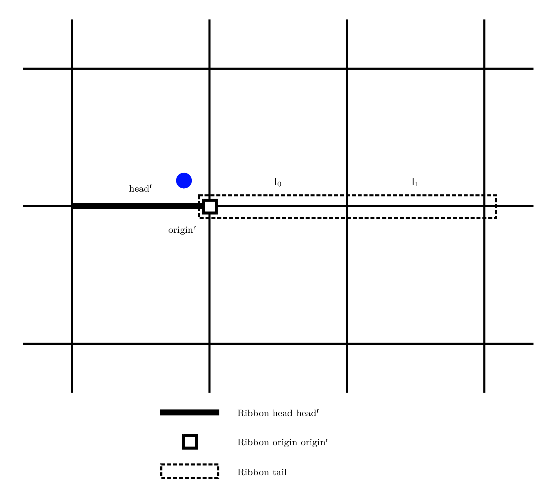
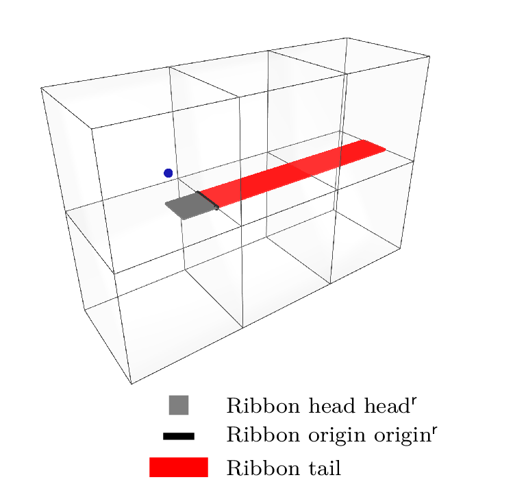
A ribbon where the tail , is composed of consecutive interfaces , originating at an origin -cell , and is the head interface that is opposite the tail . The origin -cell must be regular and interior to the mesh. We say a ribbon with interfaces in the tail is a ribbon of length . The skeleton of a ribbon, denoted by , is the array of -cells which are attached to the interfaces in the tail and parallel to the origin -cell , including the origin -cell. The fact that the definition of a ribbon is defined using -cells prevents a meaningful definition of ribbons for univariate U-splines. Fortunately, all univariate U-splines of maximal continuity are admissible and so this is not a problem.
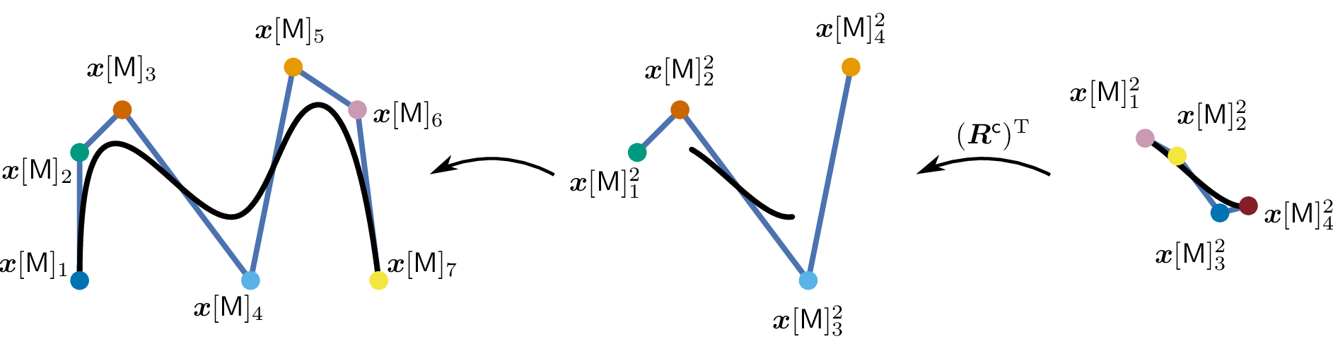
Figure 10 illustrates a ribbon composed of several consecutive interfaces in both the two- and three-dimensional mesh cases. A small solid circle or sphere near the head of the ribbon represents an initial Bernstein coefficient, adjacent to which is the origin -cell . The interfaces in the tail extend to the right. The head of the ribbon is the interface immediately opposite the tail.
Figure 10: An example of a ribbon on a two-dimensional mesh (left) and on a three-dimensional mesh (right). In each case, a small solid circle or sphere near the head of the ribbon represents an initial Bernstein coefficient.
4.4.1.1 Maximum Coupling Length
A ribbon can originate from any interior regular -cell in a U-spline mesh, and can be of any length . However, we will primarily use ribbons to measure the maximum distance, measured by the length of the ribbon, between a specified Bernstein coefficient and any other coefficient coupled to it. We call a ribbon constructed in this way a ribbon of maximum coupling length. In this case, the length of the tail is determined by how far that coefficient can couple with neighboring coefficients in the direction of an interface which is adjacent to the origin -cell (this becomes the first interface in the tail). A ribbon of maximum coupling length is said to be truncated if the length of the ribbon is shortened due to reduced continuity on the final interface encountered by the tail.
4.4.1.2 Continuity Transitions
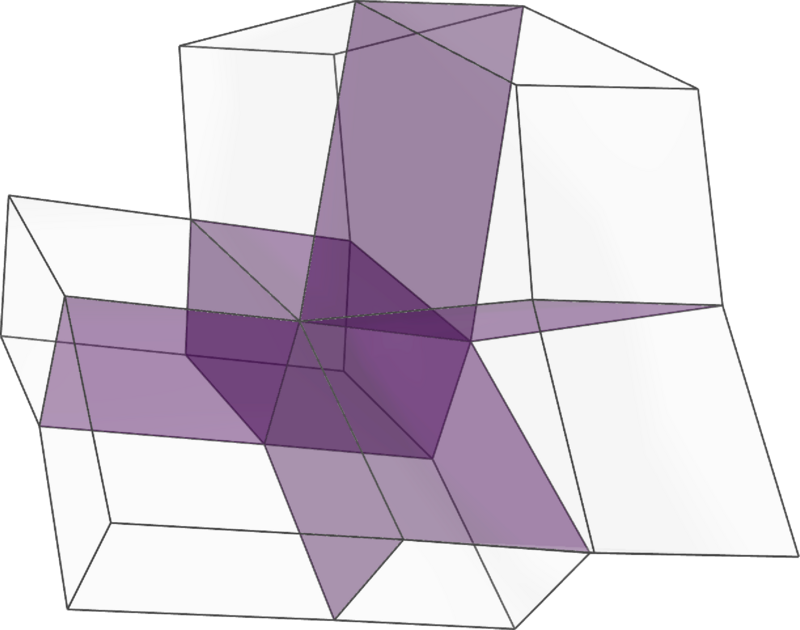
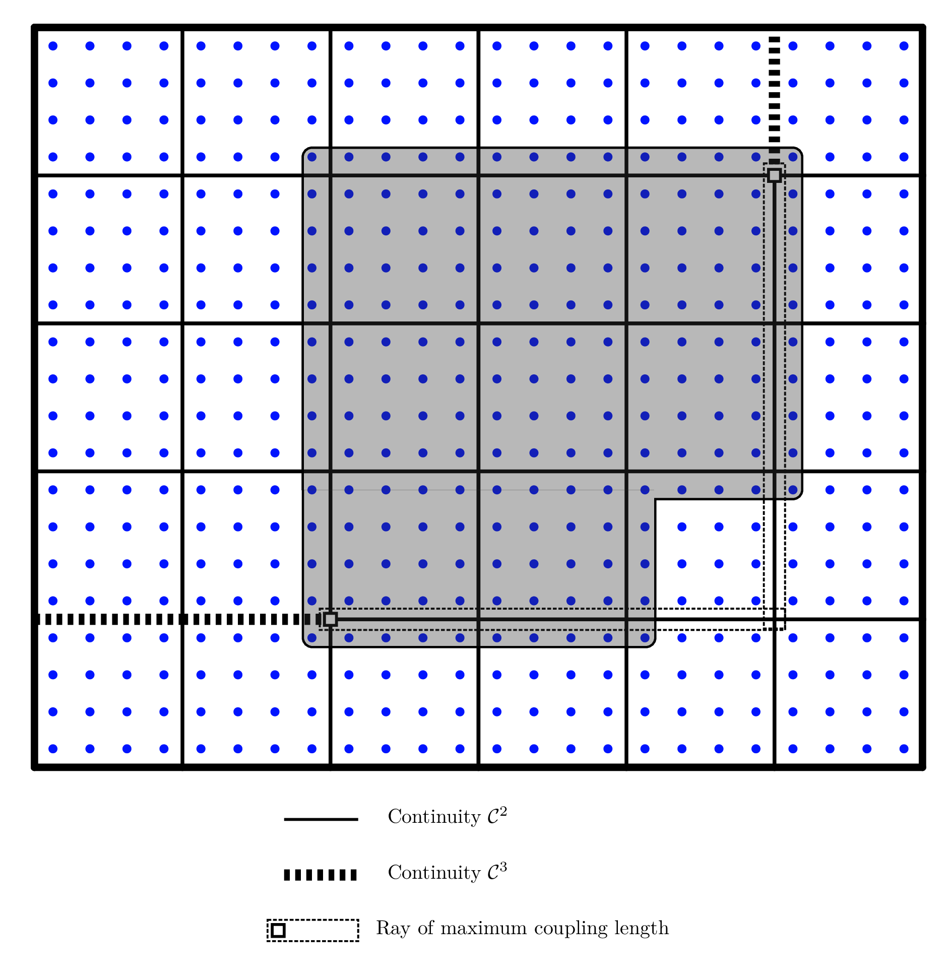
A continuity transition ribbon (designated by ) is a ribbon of maximum coupling length with the additional property that . An example of this type of ribbon for both two and three dimensions is seen in figure 11. Two perpendicular continuity transition ribbons and where and is length and is length , are said to be intersecting if they share a -cell (i.e. ). A tail-to-tail intersection occurs when the shared -cell is in and in . A head-to-tail intersection occurs when the shared -cell is in and in , or vice-versa. The minimum perpendicular degree of a continuity transition ribbon is defined as .
4.4.1.3 Degree Transitions
A degree transition ribbon (designated by ) is a ribbon of maximum coupling length with the additional property that . An example of this type of ribbon for both two and three dimensions is seen in figure 12.
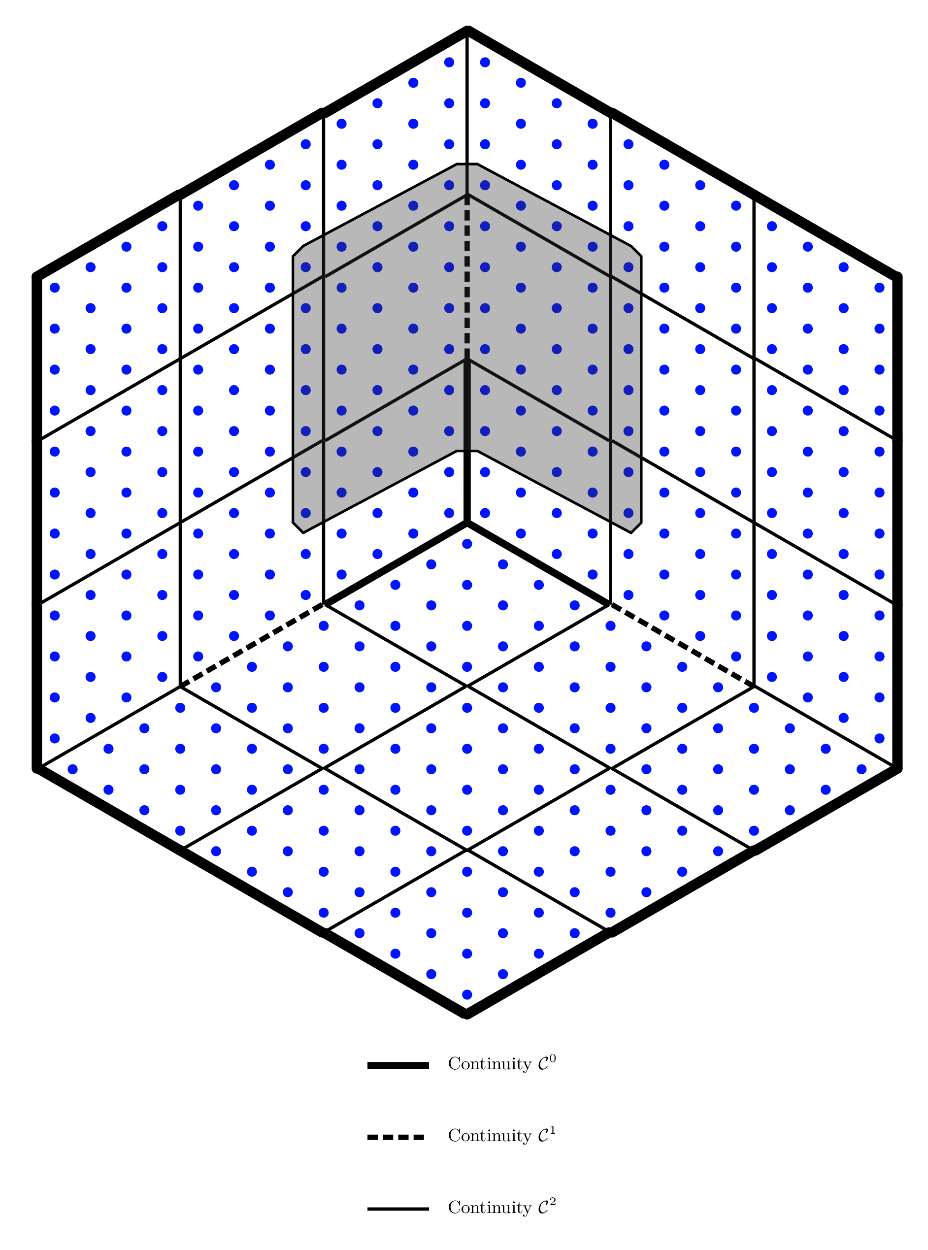
Figure 11: Continuity transition ribbons on a two-dimensional mesh (left) and a three-dimensional mesh (right). In each case, the ribbon originates at a -cell where a continuity transition occurs, and proceeds in the direction of lower continuity. All elements on both meshes are quadratic.
Figure 12: Degree transition ribbons on a two-dimensional mesh (left) and a three-dimensional mesh (right). A degree transition ribbon is a ribbon of maximum coupling length with the additional property that .
4.4.2 Admissible Layouts
As described previously, a U-spline mesh is a Bézier mesh with an admissible layout. The admissibility conditions presented here were selected for simplicity, while still ensuring that the resulting U-spline spaces possess the requisite mathematical properties. It should be noted, however, that various generalizations of these conditions exist but are significantly more complex to implement and understand so are omitted from this work. We will explore these generalized conditions in a forthcoming work. For our purposes, an admissible layout satisfies the following three simple constraints:
-separation: If two perpendicular continuity transition ribbons and intersect (that is, share a common -cell), then it must be a tail-to-tail intersection or a head-to-tail intersection. If a truncated continuity transition ribbon meets with a non-truncated continuity transition ribbon tail-to-tail, then . If two truncated continuity transition ribbons meet tail-to-tail, then .
-separation: For all continuity transition ribbons , if , then and if , then . Also, no degree transition ribbon perpendicular to may intersect , the origin of .
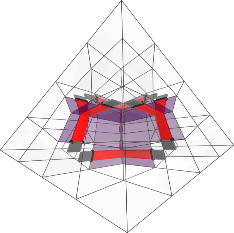
-grading: A creased -cell is any -cell in a Bézier mesh where all adjacent interfaces are creased to or . For a creased -cell and a set of continuity transition ribbons that all terminate at , and given any of length where , , then , where is defined recursively as and where and Additionally, on three-dimensional meshes, given three edges on a hexahedral element adjacent to vertex , (without loss of generality we label these edges ), if is extraordinary, then all faces adjacent to and perpendicular to and , i.e.,
must be creased. This three-dimensional requirement is illustrated in figure 18b. Note that all extraordinary -cells are required to be creased, but regular -cells may also be creased as seen in figure 14.
Examples of two-dimensional mesh layouts that satisfy the separation and grading admissibility conditions are shown in figure 13 and figure 14 and three-dimensional examples are shown in figure 15, figure 18, figure 17, and figure 16. The -separation condition is demonstrated in figure 13a and similarly in figure 15a and figure 16 where we see admissible configurations with ribbons that do not intersect except tail-to-tail or head-to-tail. We note that ribbons on volumetric meshes that cross in the middle of a face are not considered intersecting, and are admissible.
A common application of the -separation condition is seen in figure 13c and figure 15b where a transition to lower continuity must be sufficiently separated from a transition to lower perpendicular degree. Also notable is the -separation condition demonstrated in figure 13b and figure 17 where a degree transition ribbon cannot be permitted to intersect the origin of a continuity transition.
The -grading condition is demonstrated in figure 14, figure 18, figure 14, and figure 18 where we see several mesh configurations that include a creased -cell. Extraordinary -cells are always required to be creased, but the same -grading conditions also apply to the interfaces near a regular -cell if all adjacent interfaces are creased. Unstructured volumetric configurations often contain many extraordinary edges, as the hex-meshed tetrahedral topology demonstrates in figure 18a. When an extraordinary edge is near a boundary on a volumetric mesh, sometimes additional faces must be creased as is demonstrated in figure 18b. In this case, an additional face to the left of the extraordinary edge was required to be creased (despite itself being adjacent to only regular edges). This is because this face is perpendicular to an edge which, in turn, is perpendicular to the extraordinary edge (see equation ).
Figure 13: Examples of admissible layouts that satisfy - and -separation conditions. On the top left, two continuity transition ribbons meet tail-to-tail. On the top right, a degree transition ribbon is sufficently separated from a continuity transition ribbon to avoid intersection with the origin of . On the bottom, a degree transition is sufficiently separated from the head of a continuity transition ribbon so that .
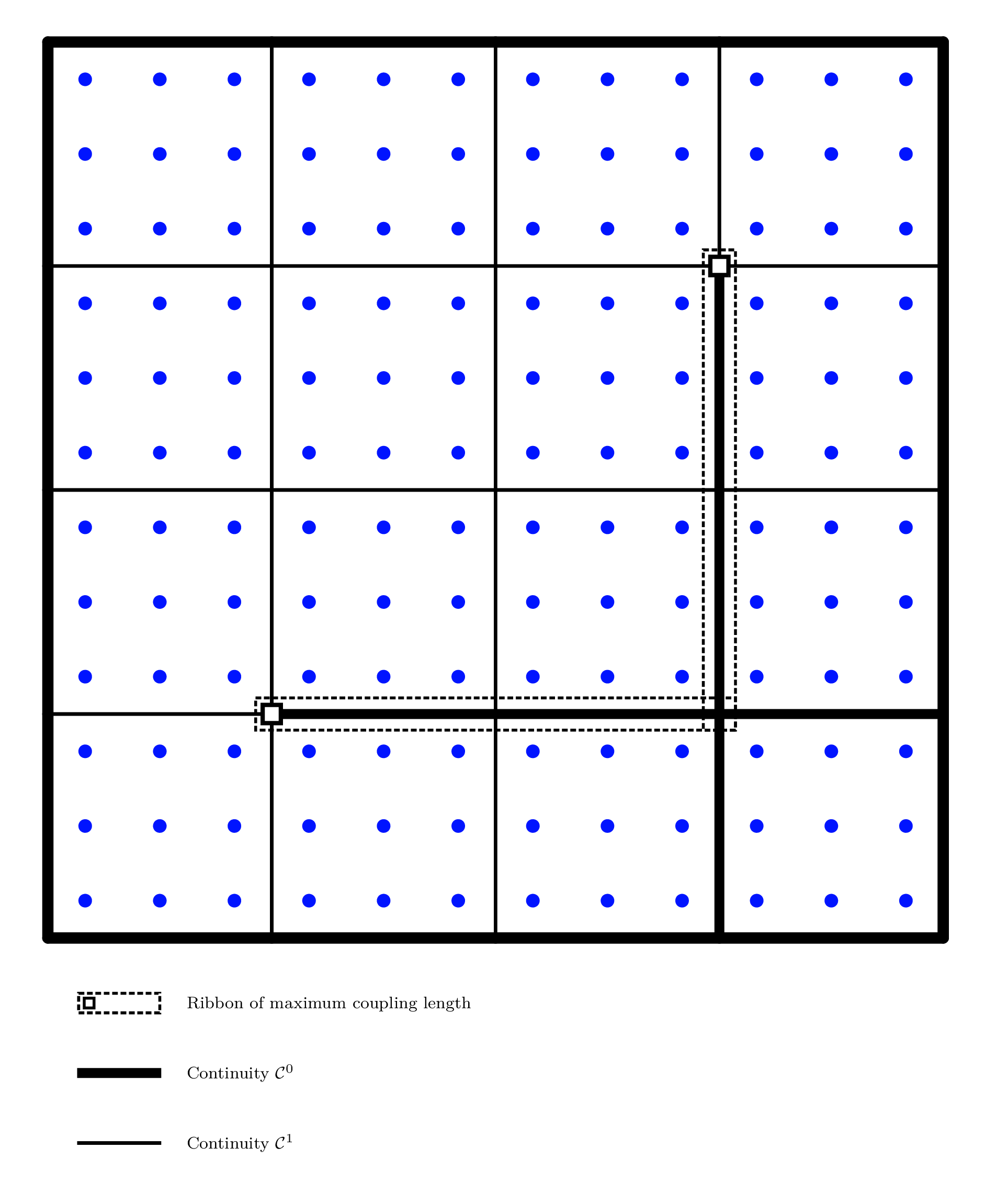
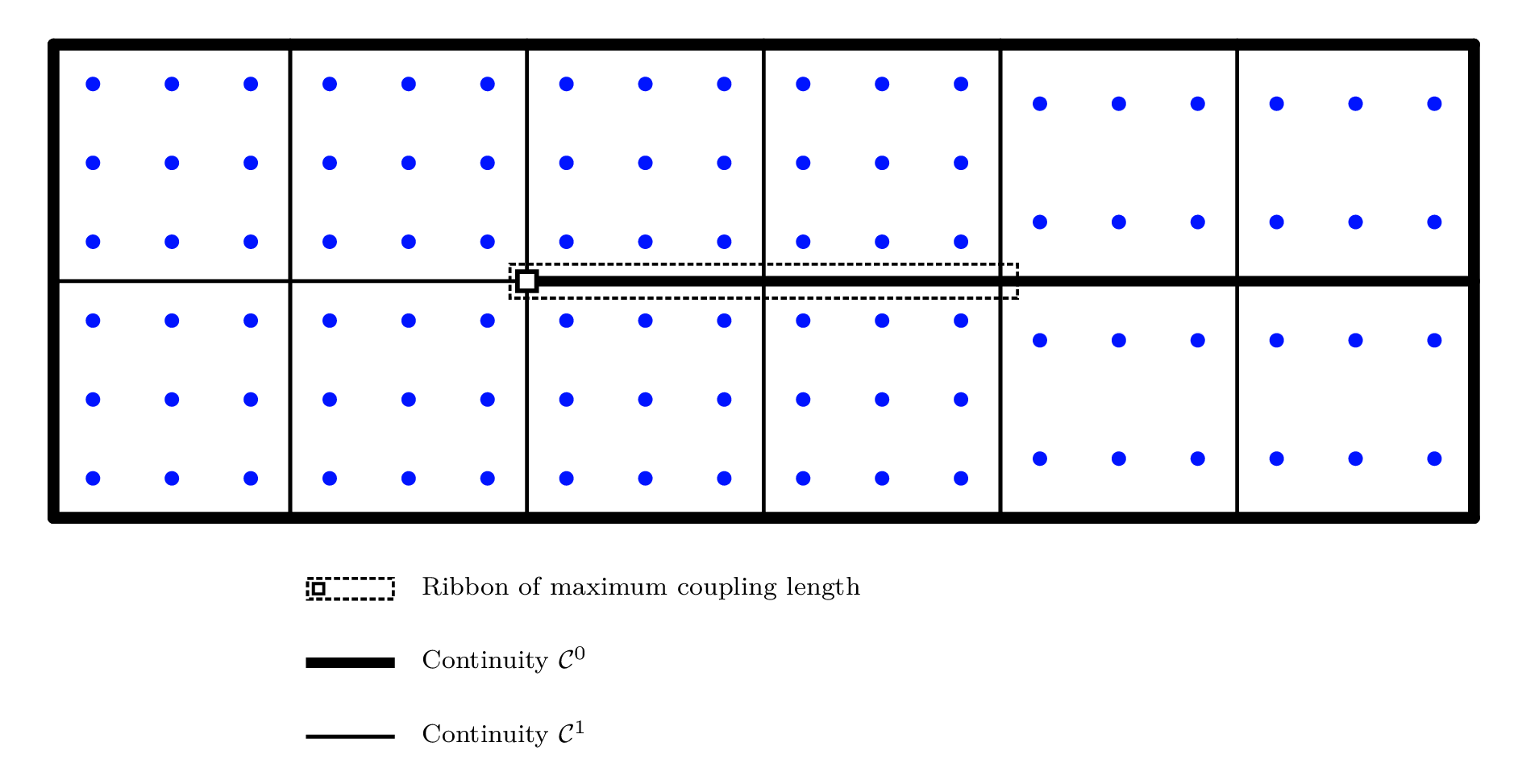
Figure 14: Example of two admissible layouts that satisfy the -grading condition. Note that while extraordinary -cells will always be creased, a creased -cell may also be regular as shown in the example on the right.
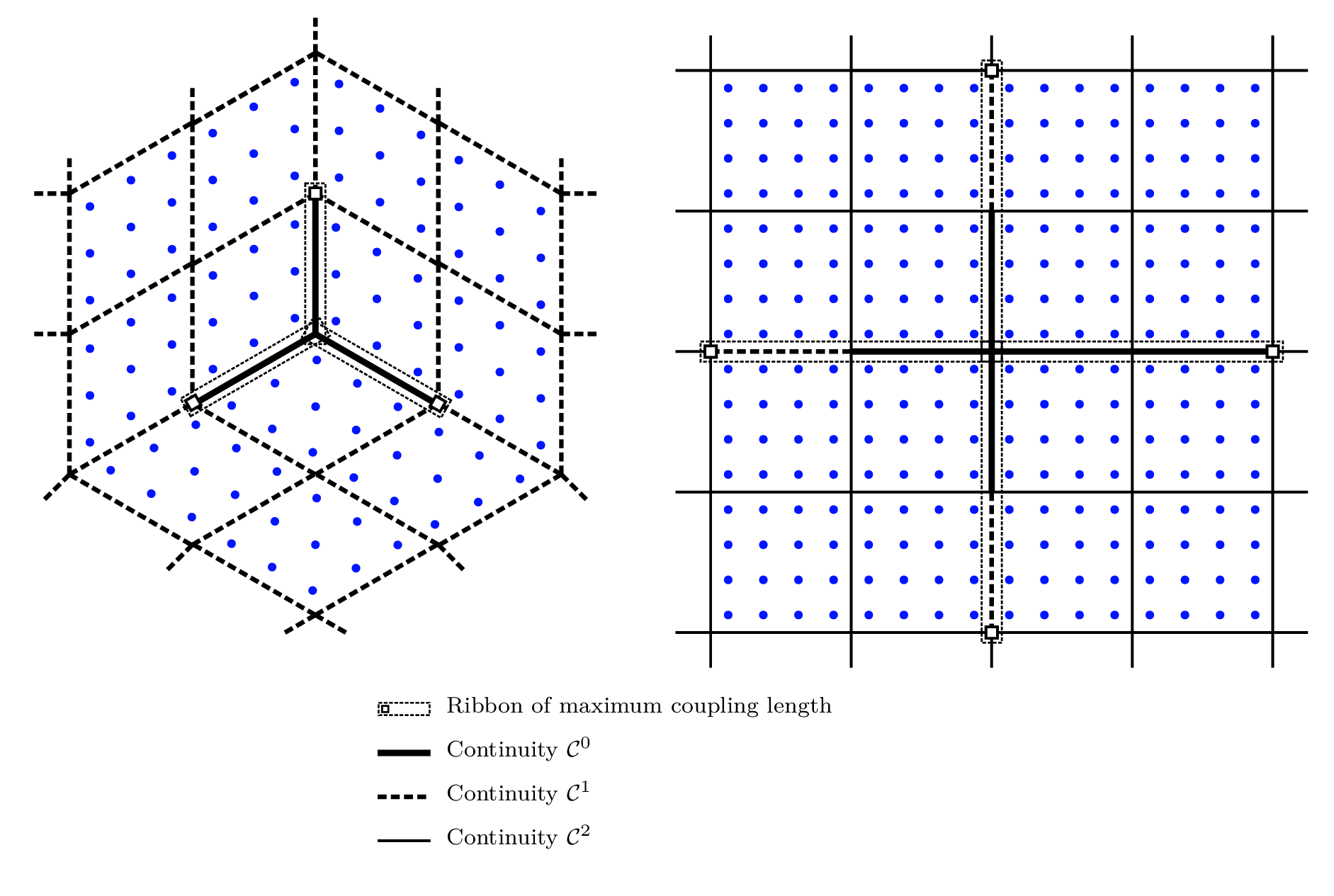
Figure 15: Examples of admissible volumetric meshes that satisfy - and -separation conditions. The example on the left contains both a tail-to-tail and head-to-tail ribbon intersection. Ribbons that cross at the center of a face are not considered intersecting and are admissible. The example on the right contains a continuity transition from to , sufficiently far from the degree transition to prevent the continuity transition ribbons from overlapping the cells with lower degree.
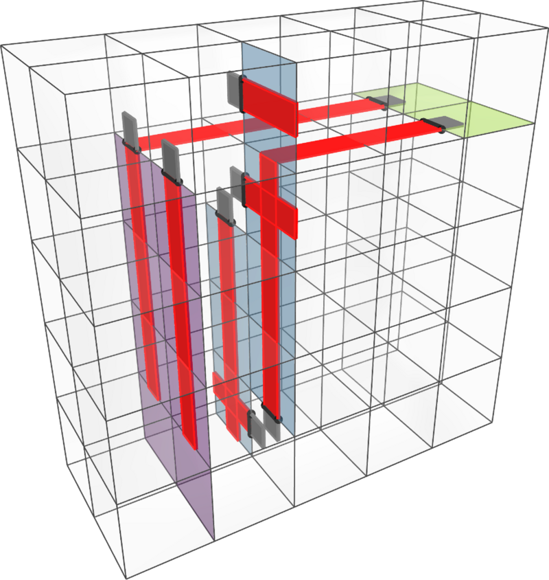
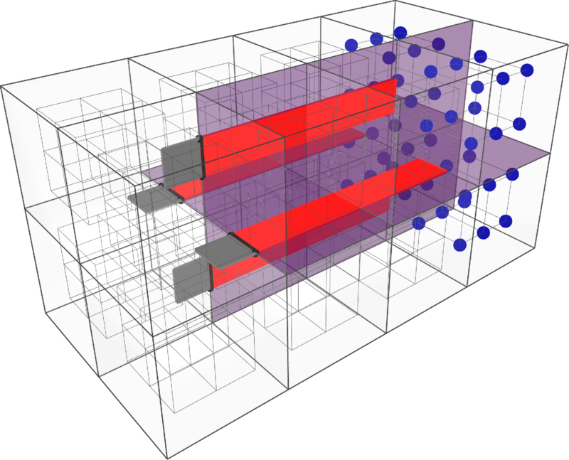
Figure 16: An example of an admissible volumetric mesh that satisfies the -separation condition. All elements are quadratic and all faces have continuity except for three mutually orthogonal planes of faces creased to . For clarity, various parts of the mesh are shown separately before they are shown together. Notice the tail-to-tail and head-to-tail ribbon intersections, which are admissible. Ribbons that cross at the center of a face are not considered intersecting and are admissible.
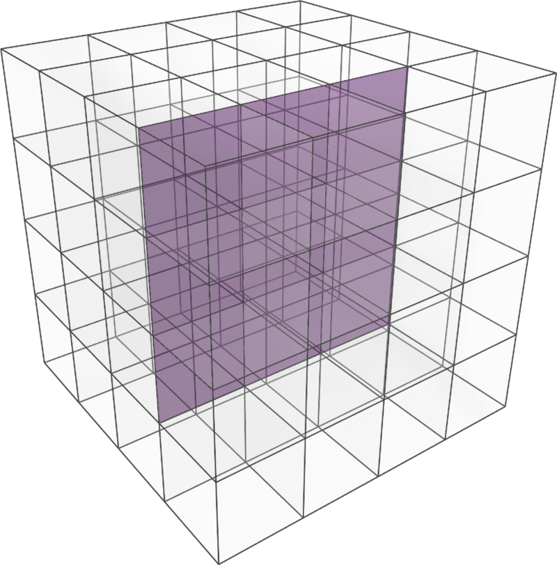
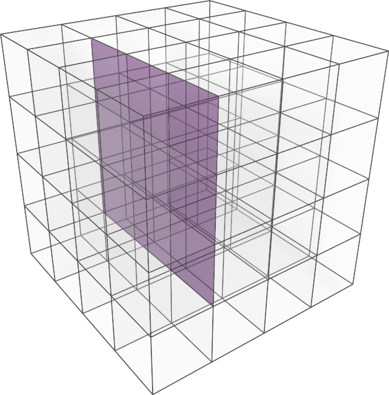
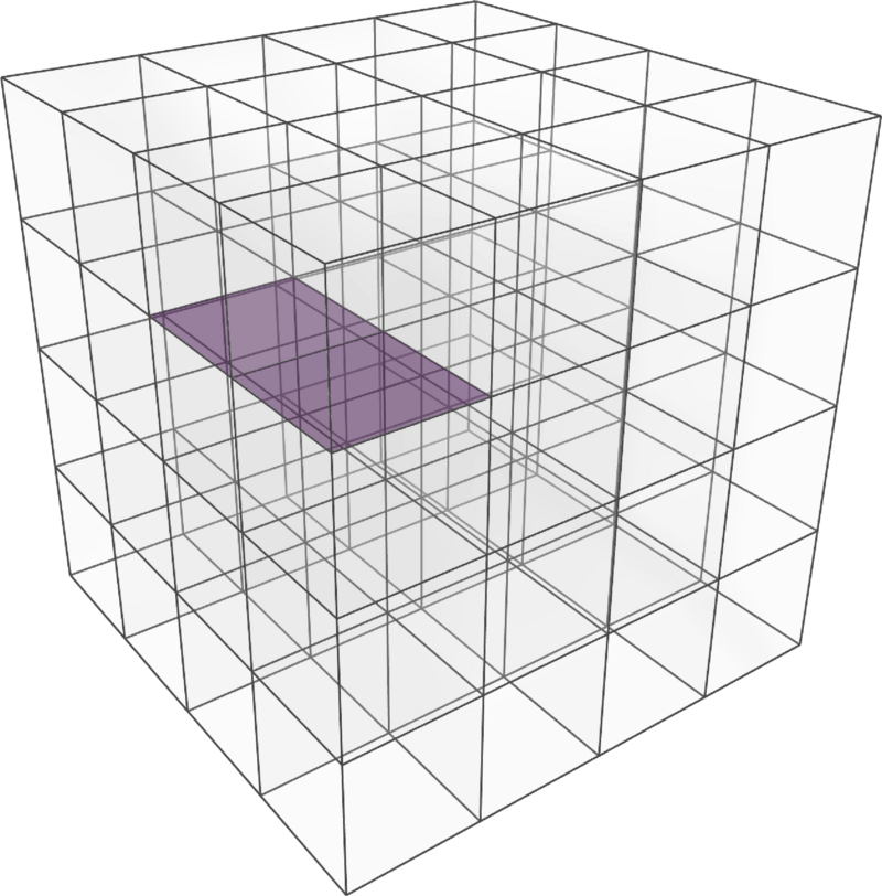
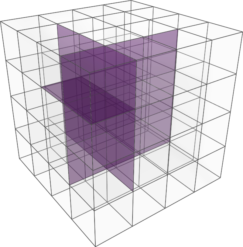
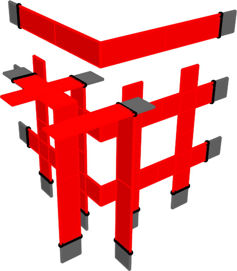
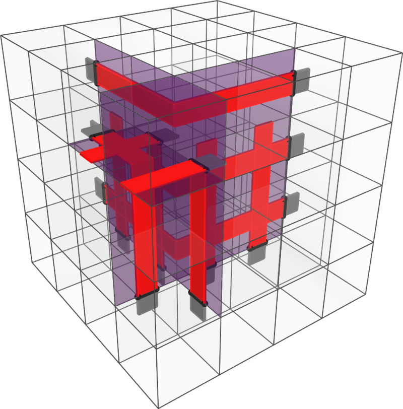
Figure 17: An admissible mesh that satisfies the -separation condition. This mesh is cubic everywhere except for five cells on the far side, which have been set to , and a few faces on the near side which are set to (supersmooth). The degree transition ribbons may be seen extending away from the cells with lower degree. Observe that these transition ribbons do not intersect the edge where a supersmooth continuity transition occurs, thus maintaining the admissibility of the mesh. Both the front view and side view of the mesh are shown.
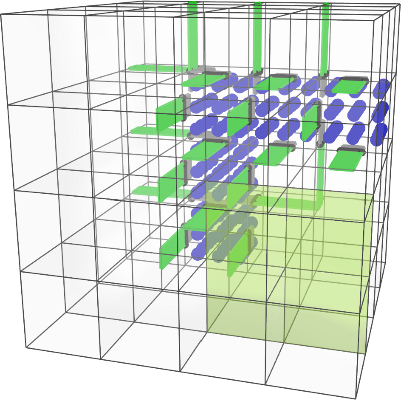
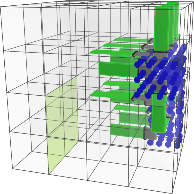
Figure 18: Two quadratic volumetric meshes that satisfy the -grading condition. The mesh on the left was constructed by filling a tetrahedron with hexahedral cells. All faces adjacent to an extraordinary edge must be creased to , but there are cases where a face near but not directly adjacent to an extraordinary edge must also be creased, as seen in the example on the right (see also equation ).
4.4.3 Classification
We denote a class of U-spline meshes by , with a superscript that is used to identify key Bézier mesh properties which are common to the meshes contained in the class (see table 2). Using this superscript notation, U-spline meshes sharing certain characteristics can be grouped and denoted by, for example , which would denote all structured U-spline meshes where variations in mesh size, smoothness, and degree propagate globally. Examples include the tensor product splines such as B-splines and NURBS. The U-spline class may not admit a global parameterization due to the possible presence of, for example, extraordinary vertices, but all variations in mesh size, smoothness, and degree propagate globally. Spline meshes in this class include unstructured finite element meshes composed of linear elements and multi-patch NURBS meshes. Analysis-suitable T-spline (ASTS) meshes are in . We note that in one dimension, the most unstructured class possible is .
In table 2, this superscript notation is related to underlying Bézier mesh characteristics.
: A global parameterization is possible.
It is possible to construct a submesh domain and an associated coordinate system on the U-spline mesh .
: A global parameterization may not be possible.
: Supersmooth interfaces are not permitted in the mesh.
All interfaces in the mesh have continuity less than .
.
: Supersmooth interfaces are permitted in the mesh.
: Smoothness propagates globally.
For any ribbon of maximum coupling length in the mesh, the continuity of the ribbon head is equal to the continuity on any interface in the tail.
.
: Local variation in smoothness is permitted.
: Polynomial degree propagates globally.
For all interfaces in the mesh, the polynomial degree parallel to the interface is the same on both cells adjacent to the interface.
.
: Local variation in polynomial degree is permitted.
Table 2: The definition of each superscript used to identify a U-spline mesh class.
4.5 The U-spline Space
Given a U-spline mesh , a U-spline space, denoted by or for short, can now be defined. As described in Splines and the Nullspace Problem, we will construct the U-spline space by leveraging the nullspace perspective for splines. However, rather than constructing and attempting to find a solution to the global nullspace problem, which can be computationally expensive and numerically unstable [22, 23], we will instead solve a single small, highly localized rank one nullspace problem for each U-spline basis function.
4.5.1 Completeness and the Neighborhood of Interaction
Because adjacent cells with differing polynomial degree can occur in admissible meshes, the notion of completeness of the U-spline basis must take into account the way a cell of lower degree affects the completeness on adjacent cells which may have a local Bernstein basis of higher degree, but only have completeness at a lower total degree, bounded by the lower degree of nearby cells.
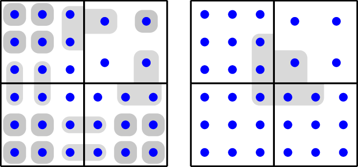
For example, in figure 19, we show a U-spline mesh with three quadratic and one linear cell, and continuity on the interfaces. The indices of the nonzero coefficients of the U-spline basis functions on this mesh are highlighted in gray. Observe that the cells directly to the left and directly below the linear cell each have a local Bernstein basis of degree , which has a total of nine functions, yet there are only eight U-spline basis functions which are nonzero on those cells. Due to their close proximity to the linear cell, these cells are complete up to degree and , respectively, or complete up to total degree . The cell diagonal from the linear cell, on the other hand, is not impacted by the linear basis and remains complete up to degree .
Figure 19: A U-spline mesh with three quadratic and one linear cell, and continuity on the interfaces. The indices of the nonzero coefficients of the U-spline basis functions are highlighted in gray. The quadratic cells on the top-left and bottom-right have a reduced degree of completeness due to their proximity to the linear cell.
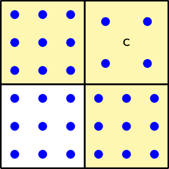
To describe this behavior, we define a submesh , called the neighborhood of interaction, of a given -cell . Let the set of basis functions that are nonzero over a -cell be denoted by and the extended support of a -cell be denoted by Additionally, we denote the set of all -cells that can be reached in a cardinal submesh direction that is orthogonal to the interfaces that are adjacent to a -cell by . Figure 20 shows for a face . Then, the neighborhood of interaction of a given -cell is defined as The neighborhood of interaction of the linear cell in the mesh in figure 19 is highlighted in figure 21. The completeness of a U-spline space is then defined as described in Mathematical Properties.
Figure 20: The faces that can be reached in a cardinal submesh direction that is orthogonal to the interfaces adjacent to , denoted by the set .
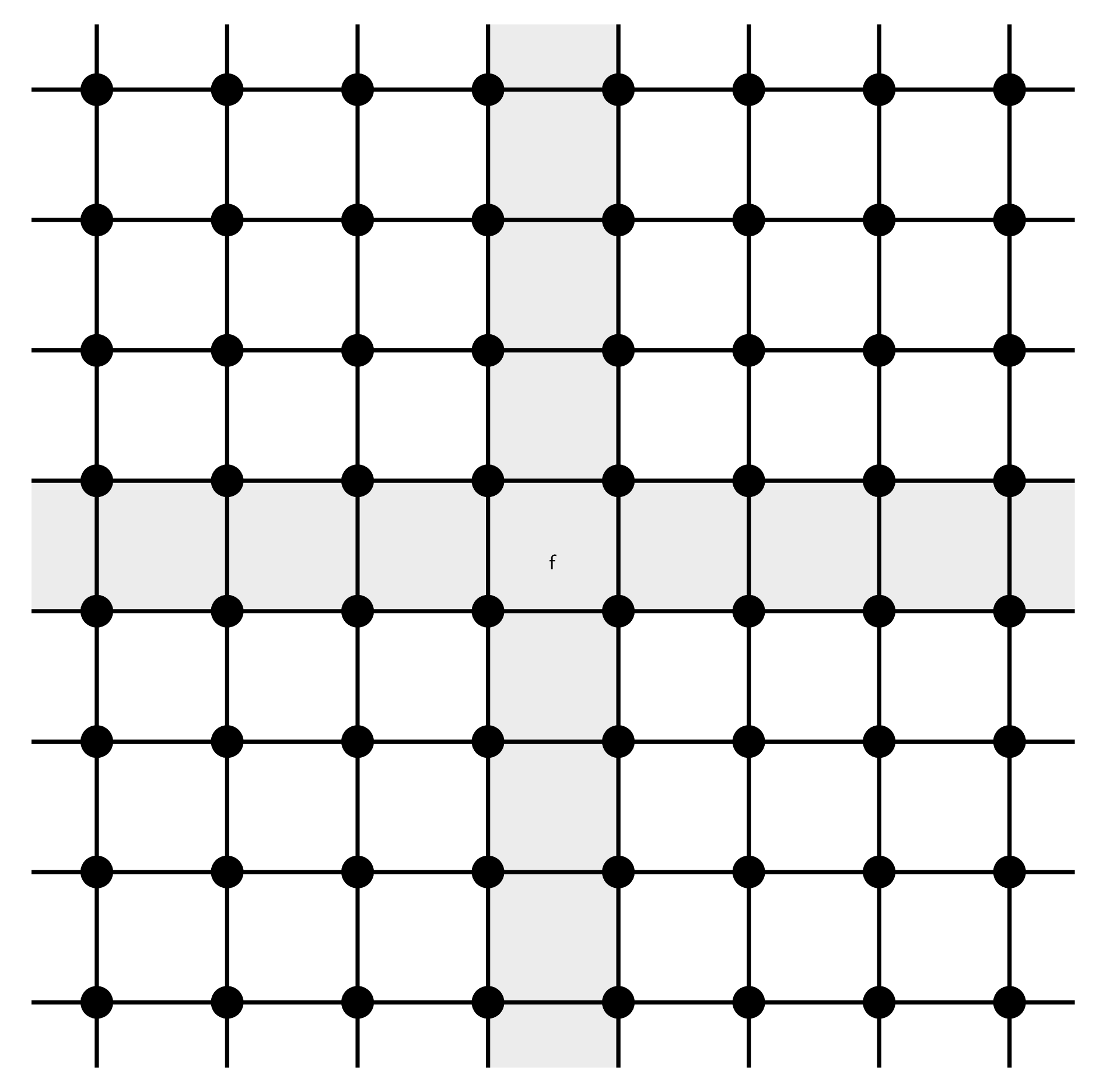
Figure 21: The neighborhood of interaction is highlighted for a cell on a two-dimensional U-spline mesh with three quadratic and one linear cell and continuity on the interfaces.
4.5.2 Mathematical Properties
Local linear independence: The set of U-spline basis functions are locally linearly independent. This means that, for any submesh , for all , where is a set of real coefficients, if and only if .
Completeness: A set of U-spline basis functions is complete through total polynomial degree over . Additionally, a U-spline space is complete through total polynomial degree over . In other words, there exists a set of real coefficients such that for any or .
Pointwise non-negativity: A set of U-spline basis functions are pointwise non-negative. More precisely, for all , where is the set of U-spline basis functions that are nonzero over .
Partition of unity: A set of U-spline basis functions forms a partition of unity. In other words, for all .
Compact support: Compact support simply means that for any U-spline basis function there exists a submesh such that for any It is desirable for the submesh to be as small as possible to preserve the sparsity of linear systems written in terms of the basis functions.
4.6 U-spline Geometry
We associate a closed subset of , called a -manifold or , for short, to every -cell in a U-spline mesh . A -dimensional manifold is constructed through an invertible mapping . The -dimensional manifold corresponding to is denoted by and is defined as Each geometric mapping or chart is defined as where is the set of U-spline basis functions that are non-zero over and is an -dimensional manifold coefficient. In a slight abuse of notation we will also call the spatial atlas and interpret it as the collection of geometric mappings or charts that cover the manifold in spatial coordinates.
-manifold
Curve
Surface
Volume
-manifold
Point
Curve
Surface
-manifold
-
Point
Curve
Table 3: The geometric terms used for manifolds of different dimensions.
We also use and to indicate both the - and -dimensional parametric manifolds and atlases, respectively, where a parametric atlas is composed of parametric charts . Note that each chart in the parametric atlas is a similarity transformation that maps between the parent and parametric coordinates of each cell in the U-spline mesh.
We call an arbitrary subdomain a segment or, if more specificity is required, we use . A set of segments is denoted by . The parametric domain of a segment is denoted by . A set consisting of all segments generated by some generic partitioning of a manifold is given by . A bounding volume of is a superset of and is denoted by while a set of bounding volumes associated with a given manifold is denoted by . The power set of an arbitrary set , denoted by , is defined as the collection of all the subsets of including the empty set and the set itself.
4.6.1 Bézier Projection
A U-spline manifold can be constructed by specifying the manifold coefficients directly or, more commonly, by computing the manifold coefficients through a geometric projection procedure. We often use Bézier projection [107] for this purpose. In the case of Bézier projection, a Bézier manifold representation of a given geometry is first computed, followed by a smoothing step to determine the final U-spline manifold representation.
Figure 22: Bézier projection is used to determine the U-spline control points for the second cell of a cubic B-spline with continuity.
We first create a Bézier manifold by constructing a Bézier mesh from the cell topology in some partition and then projecting a given geometry into the Bernstein space assigned to each cell in . This projection, denoted by , is computed for each cell as This local projection operation over each cell results in a piecewise discontinuous approximation to in Bernstein form. In other words, the map is generated such that where is the Bernstein control point associated with the th Bernstein basis function. The local projector can be chosen from a variety of options such as a least-squares projection or a local polynomial interpolation problem. The Newton-Bernstein interpolation scheme [2] is particularly efficient and robust.
To determine we apply Bézier projection to . This projection operation, denoted by , can be written as First, additional modifications may be made to to produce the U-spline mesh . The U-spline basis is constructed over in extracted form. Now, for a given cell extraction operator, defined over , the corresponding cell reconstruction operator is defined as
Using the cell reconstruction operator we can compute U-spline control points from Bernstein control points for a given cell as
Note that in most cases will be less smooth than the U-spline basis. This means the computed U-spline control points may differ from cell to cell. In this case, the global set of U-spline control points, denoted by , may be calculated from the cell-level U-spline control points using a weighted averaging scheme as described in [107]. Importantly, Bézier projection never solves a global linear system to determine the U-spline control points.
In figure 22, Bézier projection is used to determine the U-spline control points for the second cell of a cubic B-spline with continuity. The cell-local U-spline control points (center) are calculated as a linear combination of the Bernstein control points (right) through the application of the reconstruction operator . Cell-local spline control points are then mapped to the global U-spline control points (left) through an appropriate cell-to-global index map.
4.7 Notable U-spline Examples
4.7.1 Supersmooth Interface Layout
Figure 23 shows a U-spline mesh where two perpendicular continuity transition ribbons, emanating from supersmooth interfaces, touch at a common endpoint. The support of a nearby U-spline basis function is also shown. Notice the non-rectangular support of the basis function, required in this configuration to ensure local linear independence of the U-spline basis near the transition.
This example contrasts with T-splines, that leverage a type of supersmooth interface, called a T-junction, which only produce blending functions that have a tensor product structure [56, 88]. U-splines, on the other hand, are not limited to a tensor product structure, and can therefore produce an analysis-suitable basis on certain meshes which cannot produce analysis-suitable T-splines. This is particularly evident in cases where infinitely smooth interfaces are close enough in proximity to interact, as we see in this example.
Figure 23: An example of a U-spline basis function that has a non-rectangular shape due to the close proximity of two continuity transitions near supersmooth interfaces. Notice the two perpendicular transition ribbons, starting at the vertices adjacent to the supersmooth interfaces, which touch at a common endpoint. This is an example of a basis function which is not possible with T-splines, which require basis functions to have a tensor product structure.
4.7.2 Handling Degree Transitions
Figure 24 illustrates a transition from a degree , continuity section of the mesh to a degree , continuity section. The continuity in the vicinity of the degree transition must be carefully set to maintain the admissibility of the U-spline mesh.
4.7.3 Extraordinary Vertices
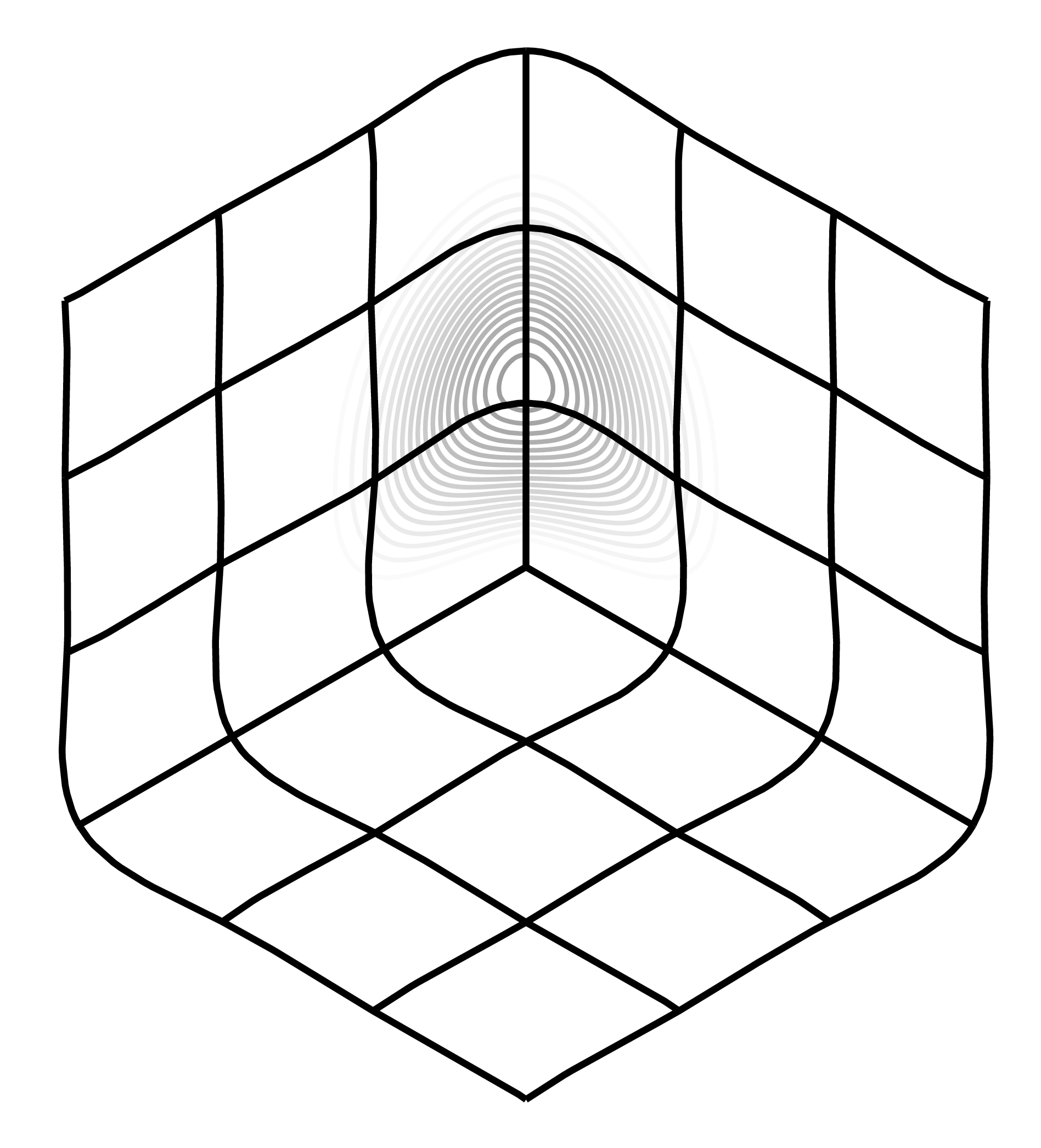
A cubic U-spline mesh that contains an extraordinary vertex is shown in figure 25a. Graded creasing on the edges emanating from the extraordinary vertex transition the continuity gradually from to . The highlighted basis function overlaps these edges, transitioning from to smoothness within its support. The control points for a linear parameterization of the mesh are seen in figure 25b, and a contour plot of the highlighted basis function is seen in figure 25c.
Figure 25: An example of a cubic U-spline basis function near an extraordinary vertex that transitions from to , and then from to .
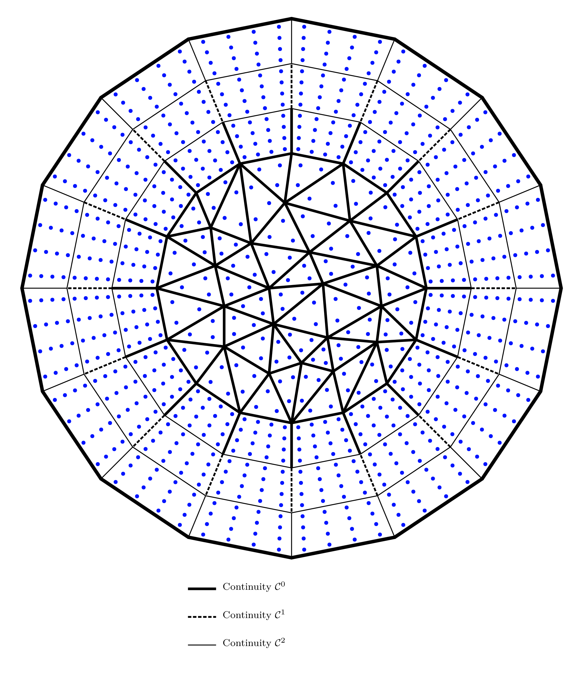
4.7.4 Triangles
In figure 26 two tensor product regions meet diagonally. Triangles are used in the transition region. In figure 27 triangles are utilized in one portion of the domain, which then interface with quadrilateral cells to transition to a outer boundary.
Figure 26: A U-spline composed of quadrilateral and triangular cells.
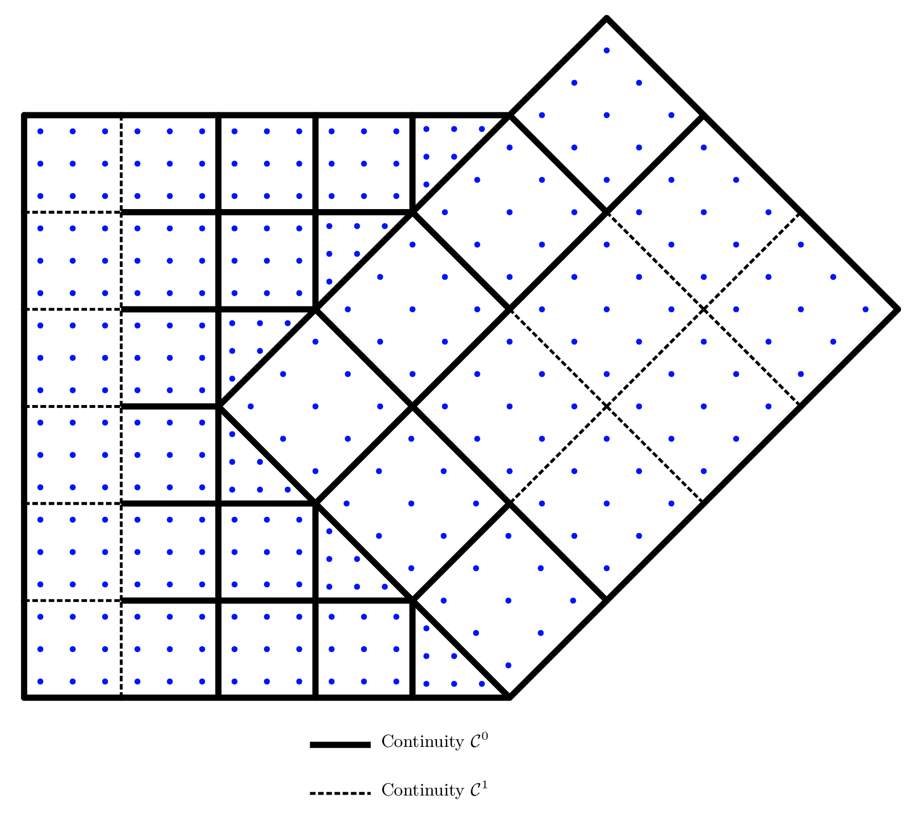
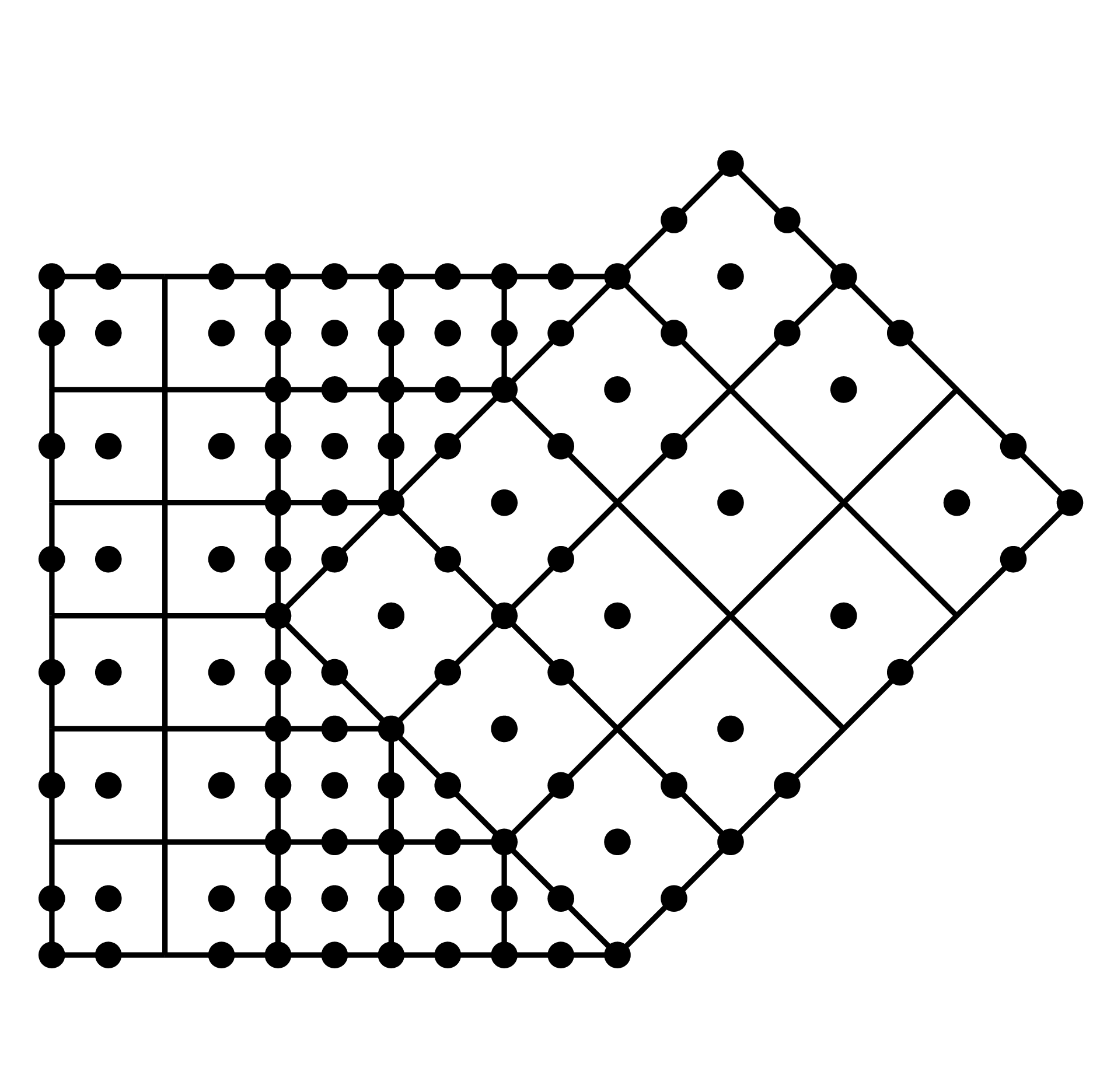
Figure 27a: This U-spline mesh is cubic with continuity on the outside edge, but is filled in the interior with linear triangles. A continuity transition was required between the triangles and the quadrilaterals.
Figure 27b: The control points and geometry of the U-spline mesh in figure 27a. Meshes of this type may prove useful to engineers who are only interested in smoothness on the surface, and opt for faster linear triangular cells on the interior.
Figure 27: A U-spline with local variation in smoothness, degree, and cell type.
4.7.5 Unstructured Volumetric U-splines
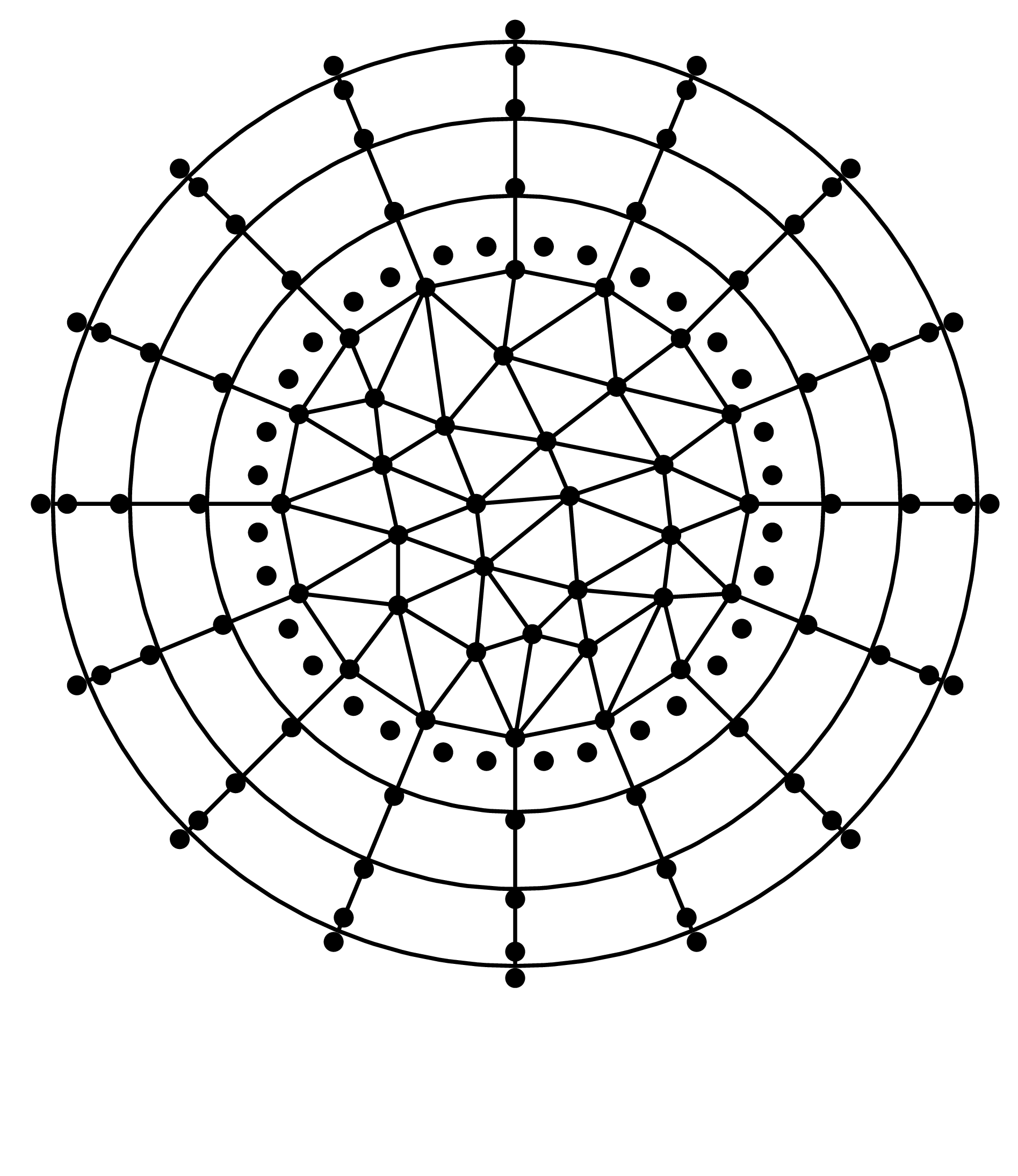
Figure 28a shows an example of a quadratic fully-unstructured volumetric U-spline mesh that forms a lattice structure with unit cells shaped like spheres with holes. This mesh has quadratic hexahedral elements. Most of the faces have continuity (colorless faces) because they are adjacent to an extraordinary edge, while a few of the faces have continuity (colored). The control points for this U-spline were chosen by projecting a linear mesh onto the U-spline basis. A rendered representation of the geometry defined by these control points is shown in figure 28b.
Figure 28a: A quadratic fully-unstructured volumetric U-spline mesh which forms a lattice structure with unit cells shaped like spheres with holes.
Figure 28b: A rendered representation of a volumetric U-spline whose basis is defined by the U-spline mesh shown in figure 28a.
Figure 28: An example of a fully-unstructured volumetric U-spline mesh. The U-spline mesh is on the left and the U-spline geometry is on the right.
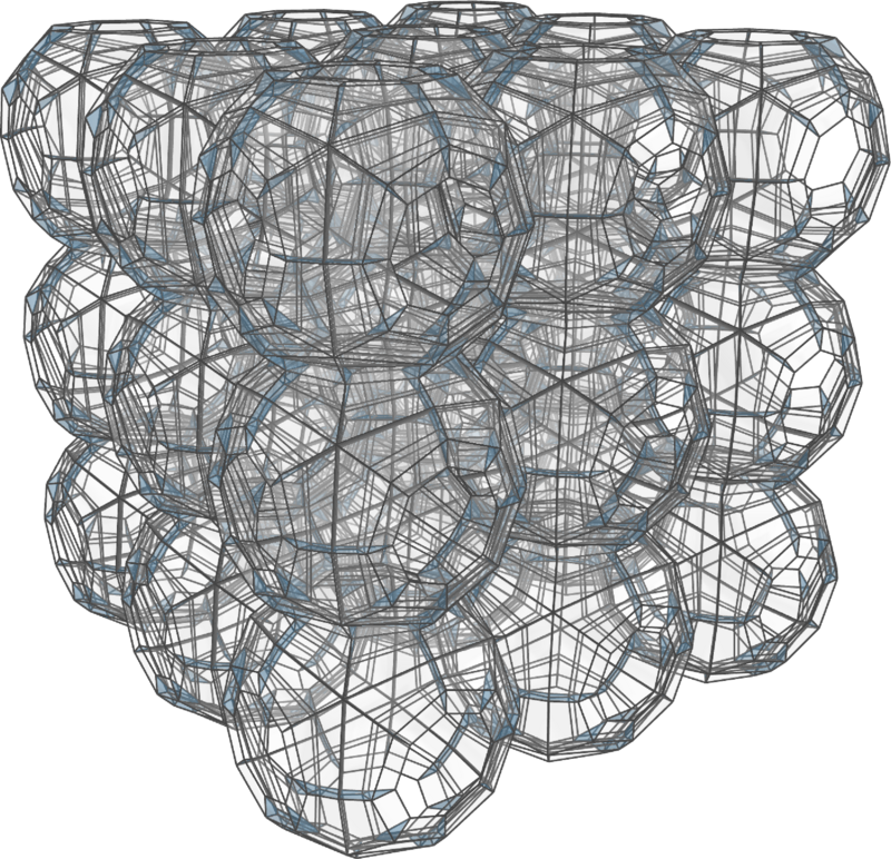
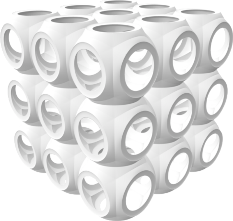
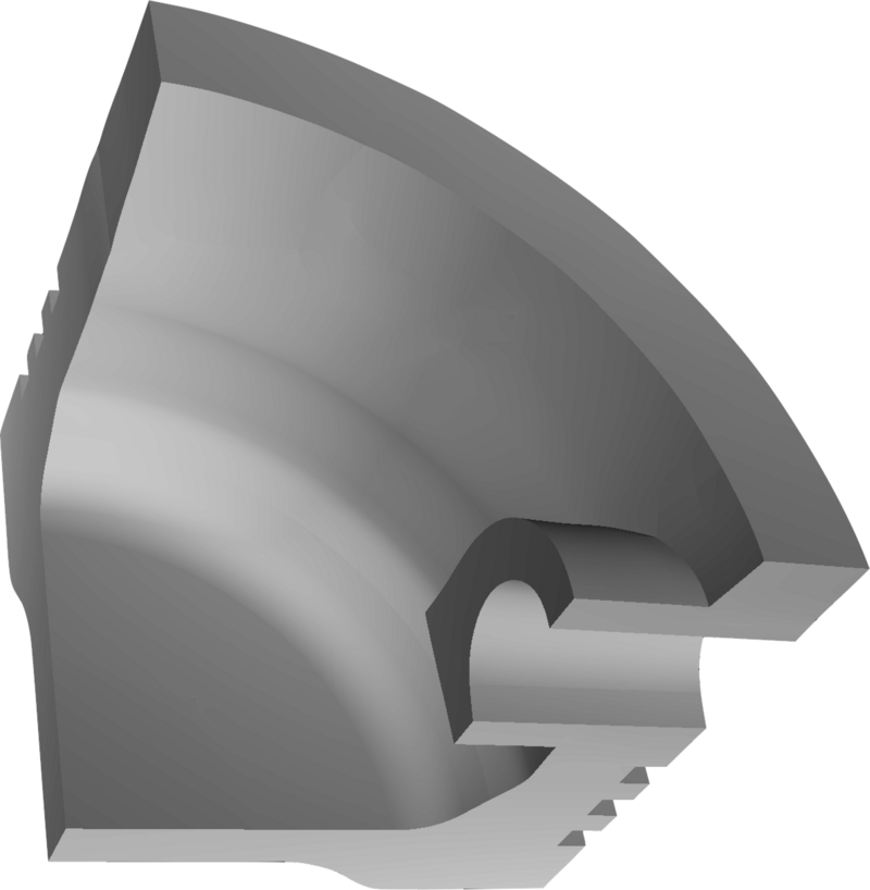
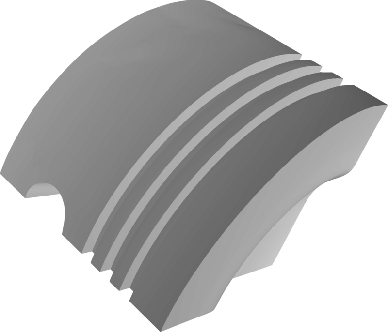
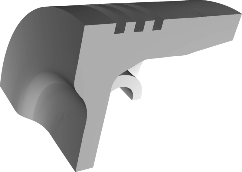
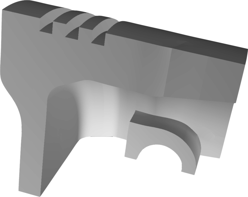
Figure 29 shows an example of a quadratic fully-unstructured volumetric U-spline mesh of a segment of a piston. This mesh has quadratic hexahedral elements. All colorless faces have continuity while the colored faces are . This example contains several extraordinary edges both interior and on boundaries. The continuity scheme set on the interfaces of this mesh uses the minimal creasing necessary to be admissible. Earlier spline methods (such as multi-patch NURBS) would have required many more faces to be creased. The control points for this U-spline were chosen by performing a projection of the linear mesh onto the U-spline basis. A rendered representation of the U-spline geometry is shown in figure 30.
Figure 29: Several views of a fully-unstructured volumetric U-spline mesh of a segment of a piston.
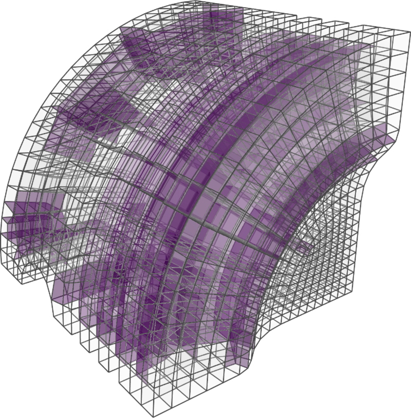
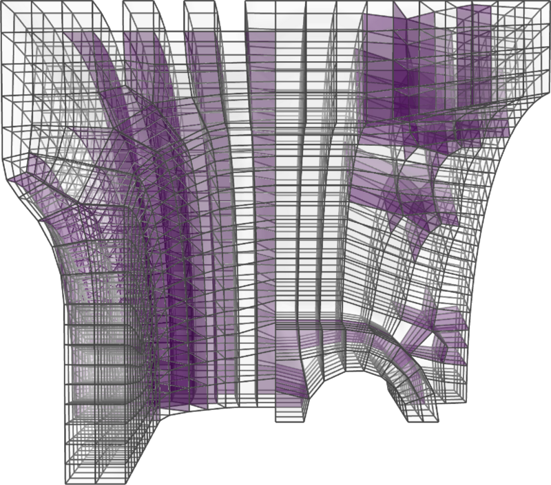
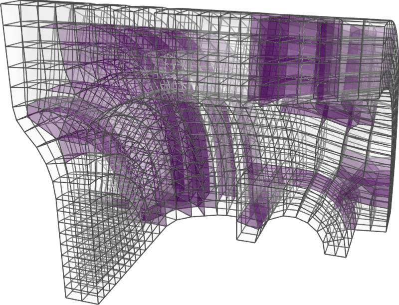
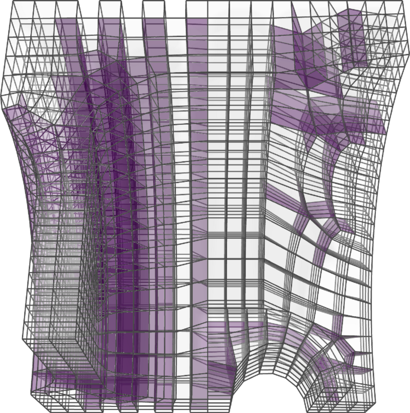
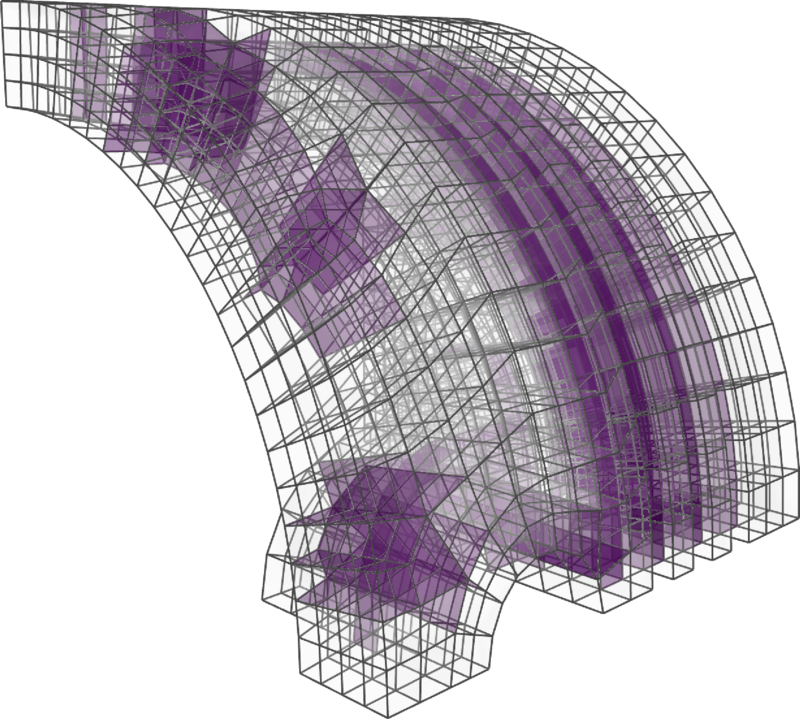
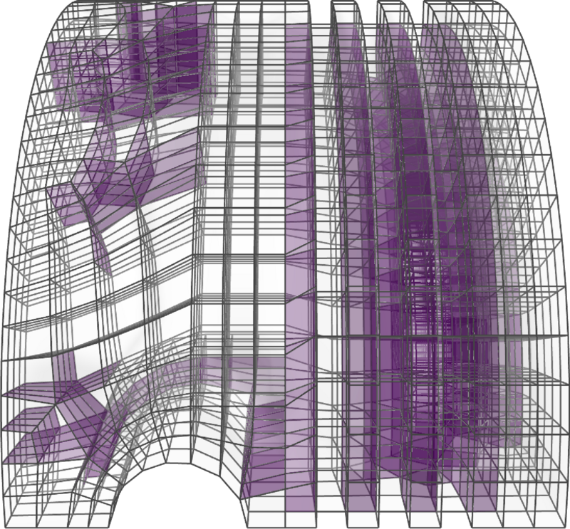
Figure 30: Several rendered views of the piston segment volumetric U-spline whose basis is defined by the mesh shown in figure 29.