5 U-splines: Construction
5.1 Bernstein basis metrics and index measurements
It will be necessary to perform various measurements on submeshes to define relationships between Bernstein bases on adjacent cells. Foundational to these techniques are the Greville points associated with the Bernstein basis functions.
5.1.1 Greville points
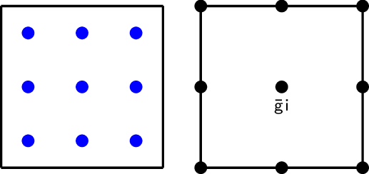
The th Bernstein polynomial on a -cell in the mesh can be associated with a parent point known as a Greville point or a domain point. For example, for a univariate Bernstein basis function of degree defined on this point or abscissa is given by and, for a tensor product function, the point is given by the ordered tuple of parent Greville points for each of the Bernstein functions appearing in the product:
An example is shown in figure 31.
Figure 31: Each Bernstein function in a cell has an associated point known as a Greville point in the parent domain of the cell, depicted on the right as small black circles.
5.1.2 Submesh domains
We now need to identify a subdomain and coordinate system that encompasses multiple cells and that allows us to easily take advantage of the ordered derivative property of the Bernstein basis defined over each cell. To accomplish this, given a submesh , a submesh domain and right-handed orthogonal coordinate system is constructed. In other words, for a given coordinate we have that where Note that the origin can be placed anywhere in but is usually placed to simplify the problem at hand. When referencing a particular submesh , we use . Note that the submesh domain corresponding to a set of indices is created by setting .
To construct we define a set of affine transformations, denoted by , , where and is a transformation composed of a scaling and a rotation . The submesh domain is now constructed as
5.1.2.1 Indexed submesh domains
The choice of the scaling operator is particularly important and can be chosen to expose certain properties of the Bernstein basis. In particular, we can define a particularly simple scaling that can be leveraged to take advantage of the ordered derivative property of the Bernstein basis. In this case, we define the scaling to be In this case, we have that and the submesh Greville points are defined by the mapping as
Due to the fact that, under the scaling chosen, all the submesh Greville points are composed of integers, we call this type of submesh domain an index domain and that the domain is indexed by the submesh Greville points . A set of submesh Greville points is denoted by and a set of sets of submesh Greville points is denoted by .
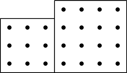
We will often choose the transformations so that both the indices and certain chosen features align. For example, when considering two cells of differing degree, the index map will not preserve all topological relationships that exist between the elements (the same vertex may be mapped to two different points under two adjacent maps, etc.) and so we choose to preserve relative orientation and require that a single vertex be preserved under adjacent maps. This is shown in figure 32. To help differentiate between Greville points on adjacent elements, we often will draw the circles representing the Greville points with respect to a scaled element inset from the boundary, as seen in figure 33.
Figure 32: The submesh Greville points on an indexed submesh domain composed of two adjacent cells with differing degree. Each Greville point is labeled with its corresponding coordinate index. The origin chosen for this submesh domain is indicated by the small axis.
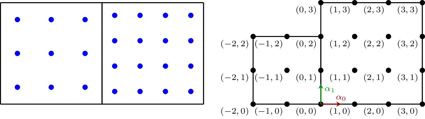
Figure 33: To help differentiate between Greville points on adjacent elements, we often will draw the circles representing the Greville points with respect to a scaled element inset from the boundary, as seen here.
5.1.3 Equivalence relations and classes
Recall that an equivalence relation partitions a set into equivalence classes. An equivalence class is a set of objects which are defined as equivalent by a given equivalence relation. The set of equivalence classes induced by an equivalence relation is commonly called a partition.
The equivalence relations used here will be based on a classical result in finite-dimensional vector spaces. Given any subspace , any vector can be written uniquely in terms of the parallel and perpendicular projectors and as
Now, given two Greville points and we define the equivalence relation to be true if and false otherwise and the equivalence relation to be true if and false otherwise. When distinguishing between parallel and perpendicular projectors is not important we will use the superscript to convey that the corresponding statement holds for either case.
These equivalence relations can then be used to create corresponding partitions of a set of Greville points denoted by . We see this in figure 34 where the Greville points on a cell are partitioned with respect to an edge using the equivalence relations and , forming partitions and . We define the shorthand and for any equivalence class we define since every point in an equivalence class has the same projected value.
We also extend the equivalence relation to sets of points. We say that a set of points is equivalent to another set of points if they project to the same set of points under the projection We can partition sets containing sets of points with this relation.
Figure 34: The parallel and perpendicular equivalence relations and are used to partition the Greville points on a cell with respect to the adjacent edge , forming partitions and .
5.1.4 Alignment
In order to compare indices on two or more adjacent elements, we define the concept of alignment. We first introduce the concept in two dimensions where an intuitive geometric description is available and then generalize those ideas to arbitrary dimensions.
5.1.4.1 Alignment in two dimensions
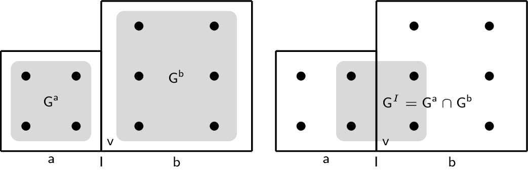
We consider two elements and on a two-dimensional mesh. In order to compare indices on and , we construct an index domain on the two elements so that a set of boundary edges that share a common vertex are aligned and so that lies at the origin. An example of an index domain satisfying these conditions is shown in figure 32. Next, we form the set of points shared between both elements under this index mapping , where are the points on element and are the points on element . Figure 35 shows an example of these sets on two adjacent elements with degrees and .
Figure 35: An example of the sets , , and on two adjacent elements and with degrees and .
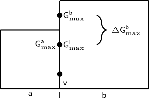
For each of the three sets , , and we determine the projected point that is farthest from : These points can be used to define difference vectors:
Figure 36 shows the projected points for the elements in figure 35 as black circles along the shared interface . The associated difference vector is shown with a curly bracket. The difference vector in this example has length zero and is not shown.
Figure 36: The projected points for the two elements in figure 35 are shown as black circles along the shared interface . The difference vector is shown with a curly bracket.
Given a difference vector we define a set of offset points given a point as Now, using to denote an axis-aligned bounding box associated with a set of points , for every point there are unique regions associated with and Each region defines a subset of the equivalence classes on the associated faces: For every there is a unique set of equivalence classes from and another unique set from . We say that these two sets of equivalence classes are aligned and define a set containing the aligned sets of equivalence classes as
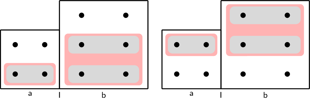
Figure 37 shows each set of aligned sets of equivalence classes for the elements in figure 35 along the shared interface . We use superscripts to refer to subsets of formed from equivalence classes associated with a single cell. is the set of equivalence classes in associated with points on . This approach may appear ambiguous for simplicial cells but because we restrict ourselves to interfaces around simplicial cells there is no ambiguity.
Figure 37: Given a Greville point on the shared interface , a set of equivalence classes on element (denoted ) is aligned with a corresponding set of equivalence classes on element (denoted ), together forming a set of aligned sets of equivalence classes (denoted ).
5.1.4.2 Alignment in arbitrary dimensions
Consider neighboring elements on a -dimensional Bézier mesh that meet at a common lower-dimensional adjacent cell . Recall that each element has a prescribed Bernstein space and set of Greville points . The cell is assigned a Bernstein space with polynomial degree equal to the minimum of all degrees on in each parametric direction parallel to . In the case that is a vertex, the Bernstein basis is assumed to be constant.
The set can be partitioned into equivalence classes with respect to as We construct trace mapping matrices for each with respect to and for each collect indices on that correspond to the nonzero coefficients on the th row of , denoted , as described in The Trace Mapping Matrix.
For each there is a unique set of equivalence classes from each defined as
We say that these sets of equivalence classes, one set from each element for a given , are aligned and define a set containing the aligned sets of equivalence classes as
As we did in the two-dimensional case, we use superscripts to refer to subsets of formed from equivalence classes associated with a single element. For example, is the set of equivalence classes in associated with points on element . In this context, we refer to as an alignment index. See figure 38 and figure 39 for simple illustrations of these ideas.
Figure 38: The concept of alignment follows naturally from the fact that multiple nonzero coefficients corresponding to higher-degree Bernstein basis functions are required to represent a single Bernstein function of lower degree (see Degree Elevation).
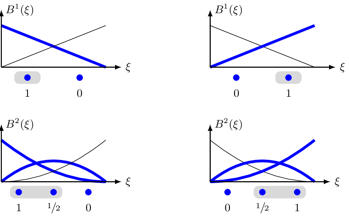
Figure 39: Given an alignment index on a shared interface , , a set of equivalence classes on element (denoted ) is aligned with a corresponding set of equivalence classes on element (denoted ), together forming a set of aligned sets of equivalence classes (denoted ).
5.2 Basis vectors for cell nullspaces
Given for any -cell we want to determine the set or system of basis vectors, denoted by , that span the nullspace of the corresponding restricted constraint matrix . Importantly, we require that a set of admissibility conditions defined in Admissible Layouts be satisfied by the mesh . With this restriction, we can use the ordered derivative property of the Bernstein basis to efficiently identify the index support of each basis vector through a series of operations on .
The set of index sets associated with a set of basis vectors is used with sufficient frequency that we use to represent it. We also define the set of mapped index sets associated with the basis vectors of the cell to be for a suitably chosen index mapping .
To aid the reader in understanding these concepts we begin in one dimension and then move to interface and vertex basis vectors in two dimensions followed last by the technical description of -cell basis vectors in arbitrary dimensions. Most of the needed intuition for the general setting can be developed in the one- and two-dimensional settings.
5.2.1 Basis vectors in one dimension
The constraint matrix to enforce across an interface in a one-dimensional mesh has rank . This is a consequence of the ordering of the Bernstein constraints. A suitable choice of permutation of the rows will produce a constraint matrix in lower triangular form and therefore the matrix has rank .
Given an interface in a one-dimensional mesh where has been assigned a continuity , the minimum number of nonzero contiguous Bernstein coefficients in any basis vector having nonzero indices in both edges adjacent to is . Let represent the row of the constraint matrix associated with the constraint for continuity of level ; there are a total of rows in the matrix. Begin with and pick a unit vector with a single positive nonzero entry that satisfies . Now pick a second unit vector with a single nonzero entry that satisfies and . The two vectors can be combined to form a new vector that satisfies . The system can be solved to find that
and so By construction, the vector has two nonzero entries. The same procedure can be applied to obtain solutions to the higher-order continuity constraints. This gives rise to the recursive definition:
where at each stage is chosen so that and so that the nonzero entry in is adjacent to the nonzero entries of . This means that each additional constraint applied adds one additional nonzero entry and so the final vector of coefficients will always have nonzero entries. At every stage there are exactly two choices for the next vector . This is due to the ordered increase in the size of constraint vectors in Bernstein form. Each constraint vector has two more nonzero entries than the previous one. Note that this construction relies on the fact that which is not established rigorously here.
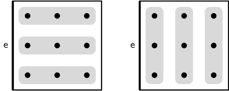
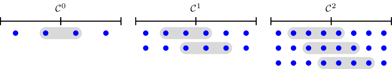
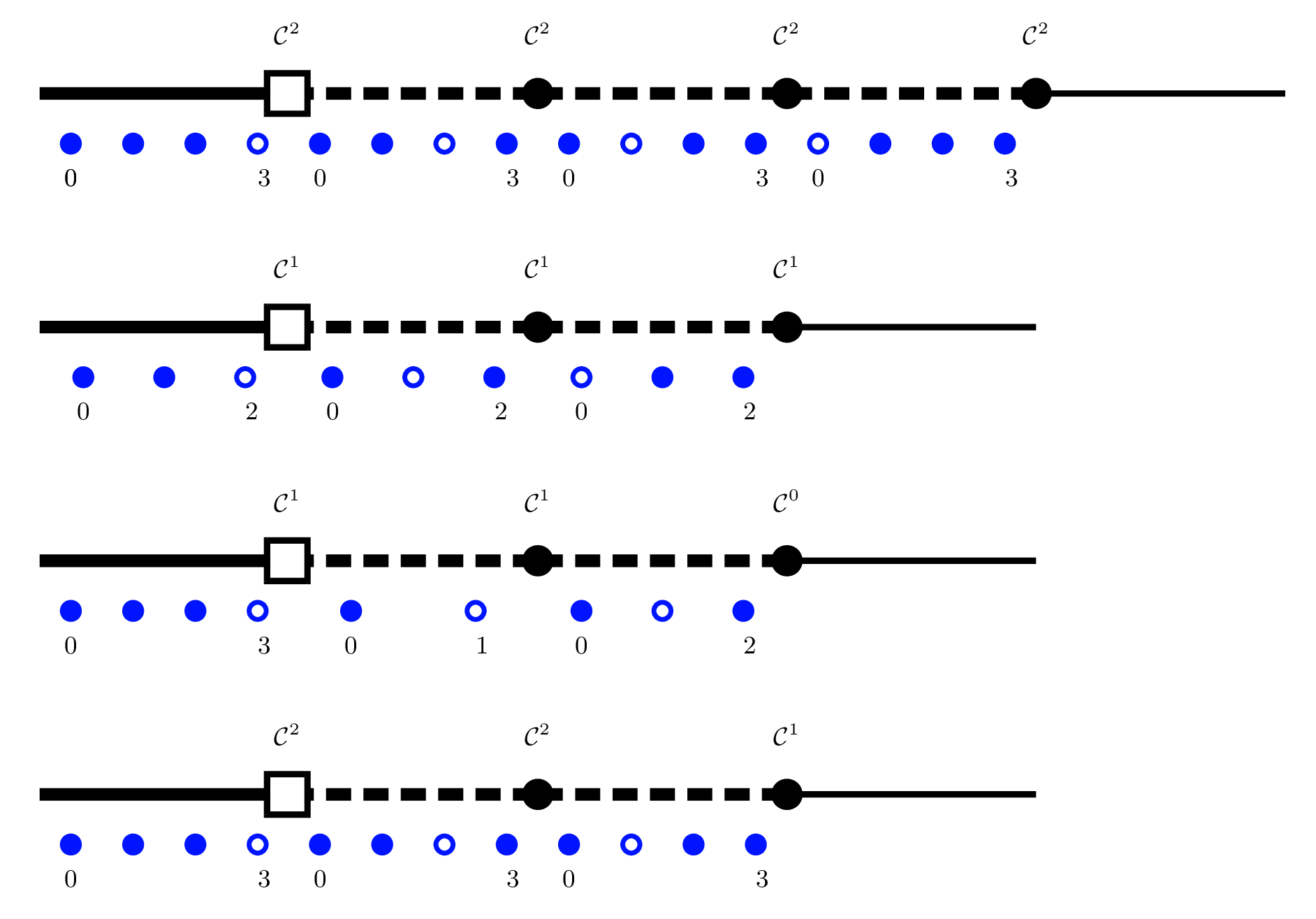
Because the number of nonzero contiguous coefficients in the basis vectors of a smoothness constraint system is given by the maximum smoothness of the system, it is possible to determine the support of the basis vectors without solving the constraint system. It is sufficient to select all unique contiguous vectors with entries that have entries corresponding to functions on either side of the interface. Examples of these one-dimensional basis vectors for various continuities are shown in figure 40. Restricting the constraint system to these nonzero entries will result in a rank one nullspace problem (see The rank one null space problem for an approach to solving rank one nullspace problems).
Figure 40: The nonzero coefficients of one-dimensional basis vectors on , , and interfaces, respectively. Each basis vector has contiguous nonzero entries.
5.2.2 Interface basis vectors in two dimensions
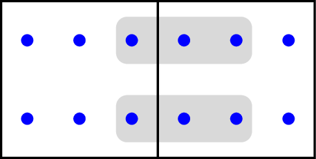
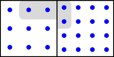
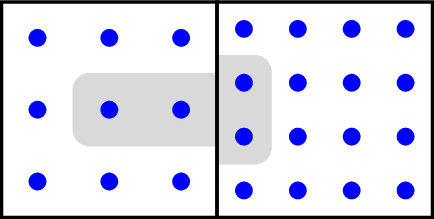
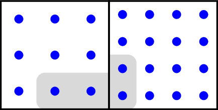
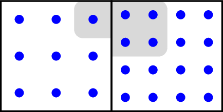
Equation can easily be generalized to an edge interface between faces with matching tensor product bases along the interface. It can be seen that the constraints separate into separate systems with exactly the same nonzero constraint values as would occur in the univariate setting repeated for each equivalence class. A simple example of a constraint matrix is given in equation . The indices corresponding to nonzero entries are highlighted with gray boxes in figure 41. In this setting, the results of equation can be applied directly to obtain the nonzero entries of each basis vector that has nonzero indices in both faces. The indices of the nonzero entries can similarly be obtained if one does not wish to solve for the values. The indices corresponding to two representative basis vectors are shown in figure 42. Each one was obtained by choosing three coefficients from a row with contiguous indices with at least one coefficient on each side of the interface.
Figure 41: Coefficients corresponding to the nonzero entries in the rows of the constraint matrix. Each grey block surrounds the nonzero entries of a pair of rows in the matrix given in equation .
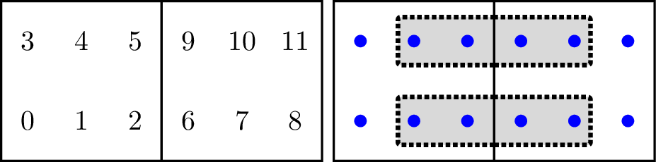
Figure 42: The indices associated with nonzero entries of two representative basis vectors for equation are shown. Each gray box indicates the nonzero entries in one basis vector.
If the Bernstein basis in each element does not match along the interface edge then the situation is significantly more complex. Consider a system consisting of two elements, one with degree and the other with degree connected by a interface such that the bases do not match on the shared interface. This is shown in figure 43. The constraint matrix is given in equation . A pictorial representation of the nonzero entries associated with each row in the constraint matrix is given in figure 43. The constraints are now fully coupled and hence the one-dimensional result may not be directly applied to compute the indices of the nonzero entries of the basis vectors.
Figure 43: Indexing convention and coefficients corresponding to the nonzero entries in the constraint matrix given in equation . The mesh has two elements with degrees and , connected by a interface. Each contiguous gray region surrounds the nonzero entries of a row in the matrix given in equation .
For every interface in a Bézier mesh there is a natural association between the equivalence classes on one side of the interface and the equivalence classes on the other side as described by equation . This association allows the results of equation to be generalized to the construction of interface basis vectors for higher-dimensional elements with local tensor product polynomial bases.
For two elements and sharing an interface with assigned smoothness and having mapped index sets and with intersection set , there are basis vectors with indices from both elements for every index in . The indices of the nonzero entries of these basis vectors are defined for all integers
For every form the sets The indices for the th function associated with are given by the union of these two sets: Once the index set has been obtained, the nonzero coefficients associated with the basis vector may be obtained by solving the smoothness constraints restricted to the index set. This also holds for interfaces between triangle-triangle or quad-triangle pairs. The set of all interface basis vectors with indices from both elements adjacent to is obtained by considering all possible values of and .
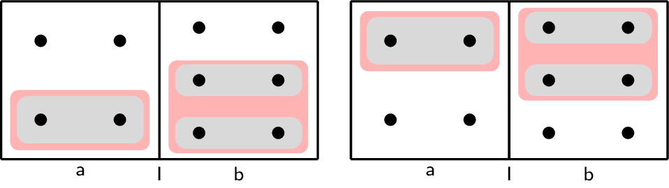
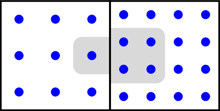
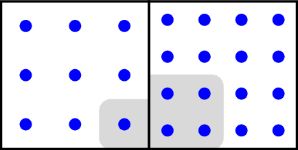
The interface basis vectors with indices from both elements in figure 43 are highlighted in figure 44. These basis vectors are in the nullspace of the constraint matrix in equation . A slightly more complex example is seen in figure 45, where two faces with degrees and are separated by an interface with continuity. The six basis vectors with indices from both faces are highlighted.
Figure 44: The basis vectors with indices from both elements adjacent to the interface. These basis vectors span the null space of the constraint matrix given in equation .
Figure 45: The basis vectors with indices from both faces adjacent to a interface. The faces have degrees and .
5.2.3 Cell basis vector preliminaries
The construction of basis vectors on -cells of dimension lower than an interface is more complex. Before proceeding with the construction of basis vectors for an arbitrary -cell we define several preliminary concepts.
5.2.3.1 Spokes and interface-element pairs
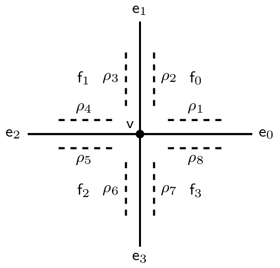
A spoke, denoted by , is a pair containing an element and an adjacent -cell , both of which are adjacent to . More specifically, a spoke is defined as Each spoke has a corresponding perpendicular interface-element pair, denoted by , and defined as In figure 46a, the spokes adjacent to a vertex are depicted as dashed lines.
We define several operations on spokes and interface-element pairs. The operator gives the interface-element pair perpendicular to a spoke on the same element and is defined as The operator gives the spoke perpendicular to an interface-element pair on the same element and is defined as The operator gives the element-interface pair on the adjacent element sharing the same interface and is defined as The operator gives the set of spokes that share the same -cell and is defined as We let .
5.2.3.2 Inclusion distances
We assign a number called an inclusion distance to each spoke, denoted , which will be used to determine the set of -cell basis vectors from each -cell adjacent to that are included in the -cell basis vector.
.
For the construction of a -cell basis vector on a -dimensional mesh, there are spokes that share each element adjacent to the -cell. We begin the process of constructing a set of inclusion distances for a -cell by choosing one of these elements and then choosing inclusion distances , one for each of the spokes on , , that satisfy the requirement . The set of inclusion distances for each -cell adjacent to are fixed by the choice of on . We denote the set of inclusion distances for all -cells adjacent to by and denote the value associated with the -cell by .
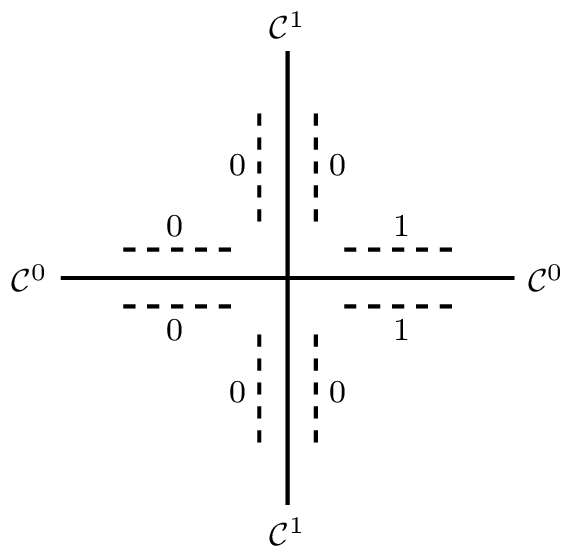
In figure 46b, a set of inclusion distances have been chosen for the spokes adjacent to a vertex , on a system where each face has a biquadratic basis, and the continuity on each edge is as indicated.
5.2.3.3 Alignment sets
We define the alignment sets on the -cell . A -dimensional Bernstein basis is placed in with polynomial degree equal to the minimum on the adjacent elements in each parametric direction to , and for each we construct the sets of aligned equivalence classes, contained in (see Alignment). For each there exists a set of -cell basis vectors such that where
5.2.4 Overview of cell basis vector construction
In general, the algorithm for constructing -cell basis vectors is recursive. It assumes the basis vectors on the adjacent -cells have already been constructed, the base case being the -cell basis vectors (the Bernstein functions). Each -cell basis vector is a linear combination of -cell basis vectors on adjacent -cells. Composite -cell basis vectors are formed by taking a linear combination of multiple -cell basis vectors, while simple -cell basis vectors are formed from just one -cell basis vector.
Construct the basis vectors on adjacent -cells by calling this algorithm recursively. The base case is a -cell, where the basis vectors are the Bernstein functions which span the Bernstein space assigned to the element.
- Composite basis vectors are constructed by considering all possible sets of inclusion distances (Inclusion distances) and all possible alignment indices (Alignment sets) on . For each,
Collect the set of -cell basis vectors associated with the given set of inclusion distances and alignment index. (Composite vertex basis vectors, Composite cell basis vectors)
The index set of the new -cell basis vector is the union of the index sets of this collection of -cell basis vectors.
Each simple -cell basis vector is constructed from a single -cell basis vector on an adjacent -cell, one for each -cell basis vector whose index set is not a subset of a composite -cell basis vector (Simple vertex basis vectors, Simple cell basis vectors).
If desired, once the index set for each -cell basis vector has been obtained, the constraint system can be solved to obtain the coefficient values and construct the basis vector.
5.2.5 Vertex basis vectors in two dimensions
We illustrate the algorithm by constructing two-dimensional basis vectors on vertices. The algorithm for arbitrary dimensions is found in Basis vectors in arbitrary dimensions. Examples of -cell basis vectors of various dimension, on both two- and three-dimensional meshes are seen in figures 50, 56, 55, 54, 53, 52, and 51
5.2.5.1 Composite vertex basis vectors
The composite basis vectors on a vertex are formed from multiple adjacent edge basis vectors. Each composite vertex basis vector is associated with a set of inclusion distances (Inclusion distances) and alignment index (Alignment sets). In the case of a vertex, there is only one alignment index. The spokes (Spokes and interface-element pairs) in this case consist of every edge-face pair adjacent to the vertex . In figure 47a we see a two-dimensional mesh with four elements. A set of spokes on the edges adjacent to the center vertex are depicted in figure 47b. We assign an inclusion distance to every spoke adjacent to the vertex , as described in Inclusion distances, beginning with two initial inclusion distance choices denoted and (corresponding to the spokes and , respectively), that satisfy the requirement . The inclusion distances associated with every spoke adjacent to , denoted , are fixed by the choice of and , as determined by the properties of inclusion distances outlined in Inclusion distances. One possible set of inclusion distances for the mesh in figure 47a is shown in figure 47c. The inclusion distance associated with a particular edge is denoted by .
We place indexed submesh domains over each pair of elements adjacent to each edge adjacent to (with their origins at ), and partition the mapped index sets of the basis vectors associated with each edge into equivalence classes with respect to the equivalence relation on the edge . We then identify the equivalence classes for which the minimum projection onto the edge is less than or equal to : An example of these equivalence classes is shown in figure 48.
Let , and . ( is defined in Adjacencies. ) We form the sets containing all indices whose associated cell is adjacent to and whose associated submesh Greville point is a part of elements of and We form the set of Greville points that are fixed points of the projectors onto or : We take all basis vectors whose projections onto the edges perpendicular to lie in : In figure 49, we see an example of these basis vector subsets marked with dotted lines.
The set of indices associated with is The full set of indices associated with and is In the case of a vertex, there is only one alignment index, so the set represents the index set of the composite basis vector. Note that for higher-dimensional cells, one additional step is required to find the set associated with a given alignment index and inclusion distances (see equation in Composite cell basis vectors).
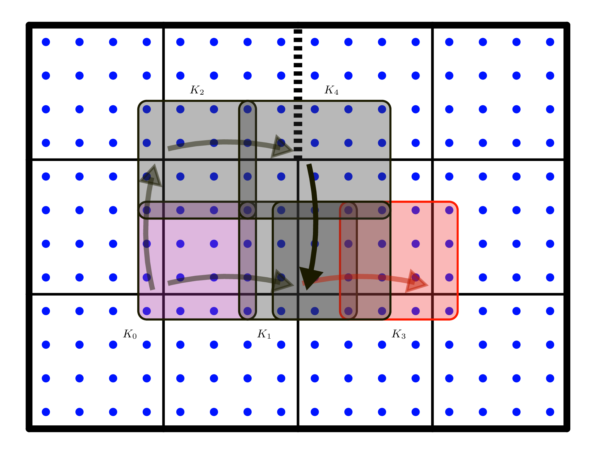
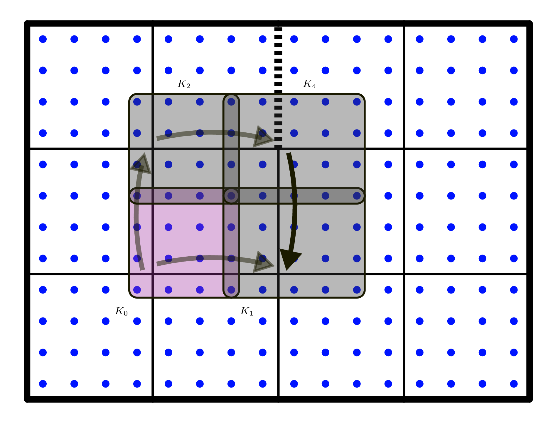
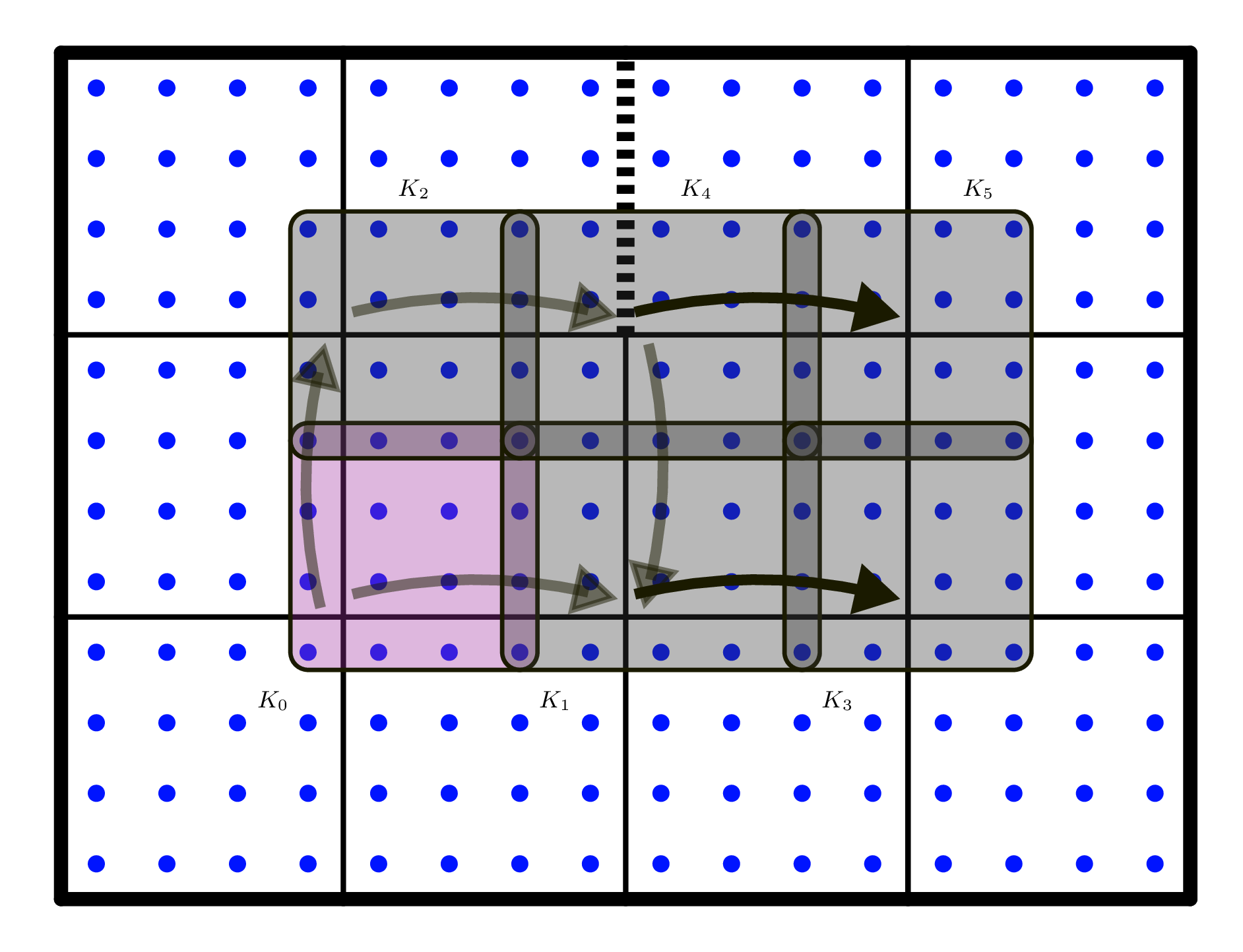
We consider all possible values of and on to construct the set of all composite vertex basis vectors. We use to represent this set. The full set of indices contained in this set is An example of a set of composite vertex basis vectors is shown in figure 50.
5.2.5.2 Simple vertex basis vectors
Each simple vertex basis vector is formed from a single edge basis vector on an adjacent edge, one for each edge basis vector whose index set is not subsumed by . We use to represent this set: An example of a set of simple vertex basis vectors is shown in figure 51.
5.2.5.3 The full set of vertex basis vectors
The full set of vertex basis vectors is found by combining the set of composite vertex basis vectors with the set of simple vertex basis vectors: Once the index set for each vertex basis vector has been obtained, the constraint system can be solved to obtain the coefficient values and construct the basis vector.
Figure 47: Choosing an initial element and two initial spokes and , and choosing the inclusion distances which uniquely identify a vertex basis vector. The fully constructed basis vector is seen in figure 50b.
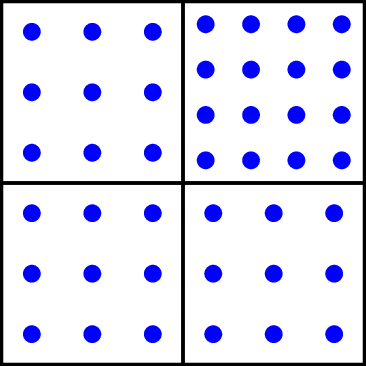
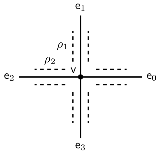
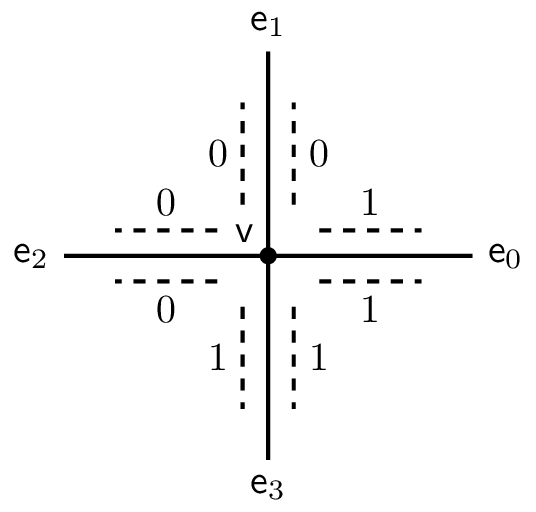
Figure 48: The basis vectors contained in for each edge , the sets of equivalence classes for which the minimum projection onto the edge is less than or equal to . Overlapping regions are depicted with darker gray. The fully constructed basis vector is seen in figure 50b.
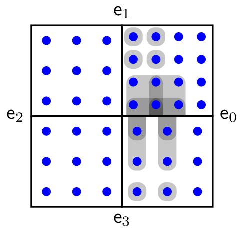
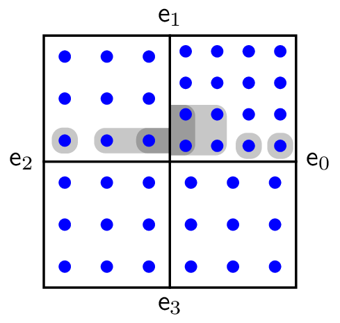
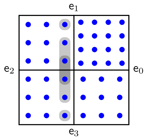
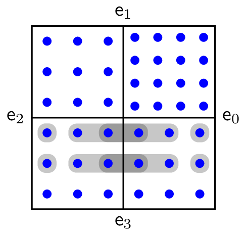
Figure 49: The basis vectors contained in for each edge . The dotted line represents the span of indices whose projections onto the edges perpendicular to lie in . Overlapping regions are depicted with darker gray. The fully constructed basis vector is seen in figure 50b.
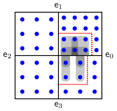
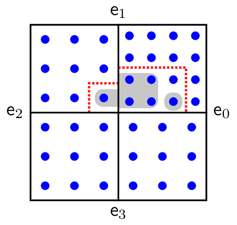
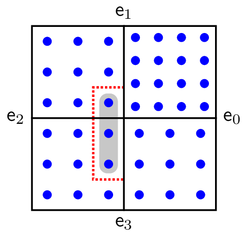
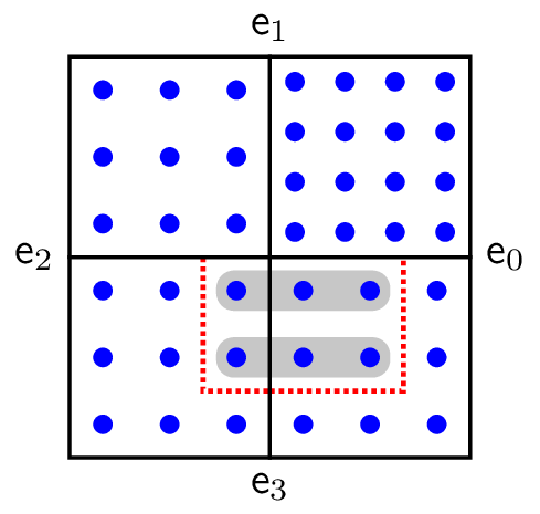
Figure 50: The composite basis vectors on a vertex adjacent to four quadrilateral cells, three with degree and one with degree . The continuity on the interfaces is .
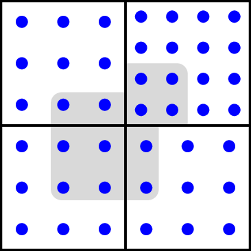
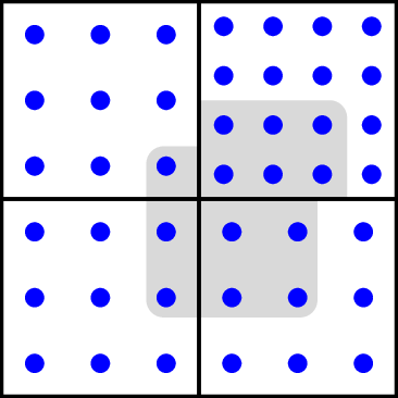
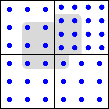
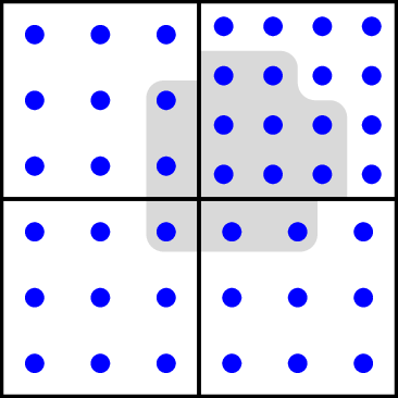
Figure 51: The simple basis vectors on a vertex adjacent to four quadrilateral cells, three with degree and one with degree . The continuity on the interfaces is . Overlapping regions are depicted with darker gray. Each simple vertex basis vector is constructed from an adjacent edge basis vector that is not subsumed by a composite vertex basis vector.
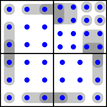
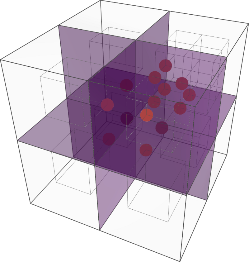
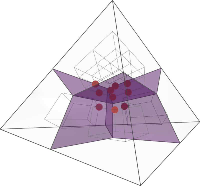
Figure 52: Examples of composite basis vectors on extraordinary vertices. On the left we see a valence three extraordinary vertex where all the cells have degree . On the right we see a valence five extraordinary vertex where some cells have degree and others have degree . In each case, the continuity of each edge is .
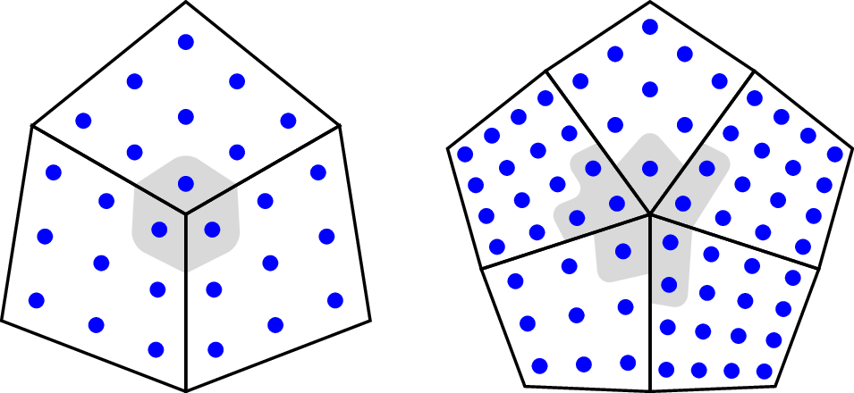
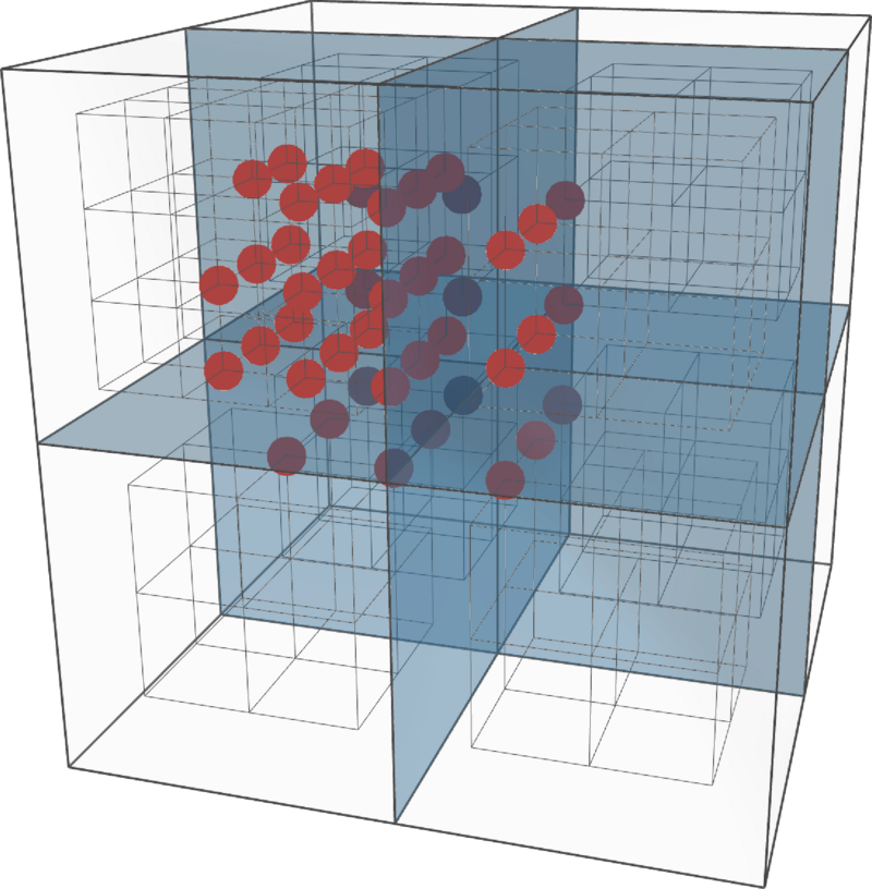
Figure 53: Basis vectors on a interface between two hexahedron on a volumetric mesh. The element on the left is linear and the element on the right is cubic. This results in four alignment sets, and one interface-overlapping basis vector per alignment index.
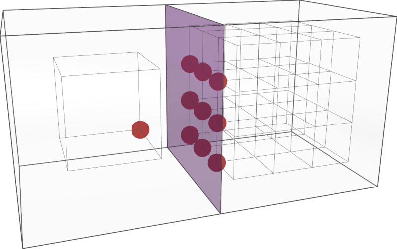
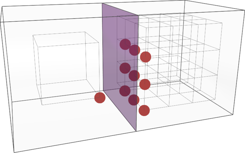
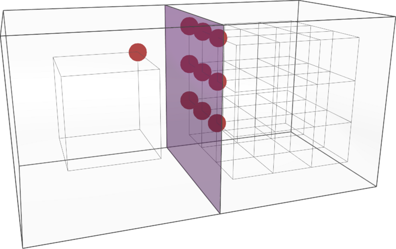
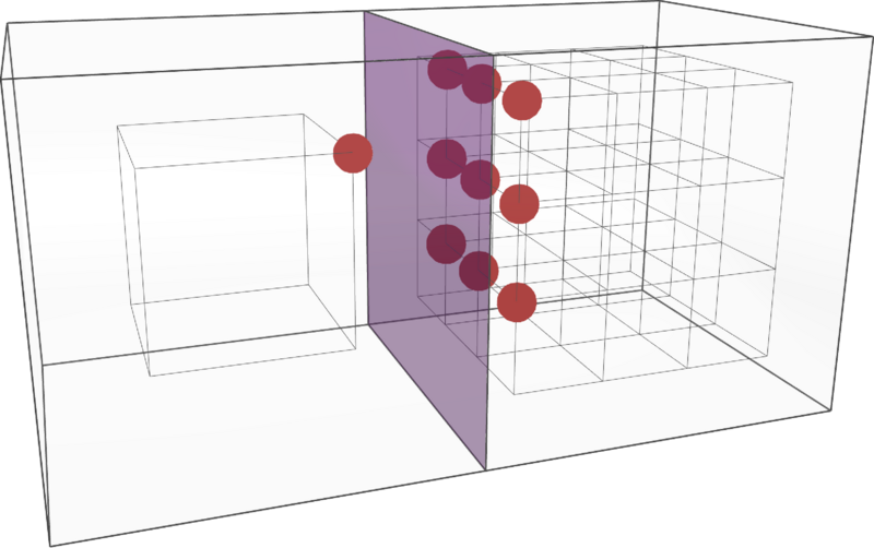
Figure 54: Basis vectors on a interface between two hexahedron on a volumetric mesh. The two elements are each quadratic in the direction normal to the interface, and then are given degrees and , respectively, in the directions to the interface. This results in four alignment sets, and two interface-overlapping basis vectors per alignment index.
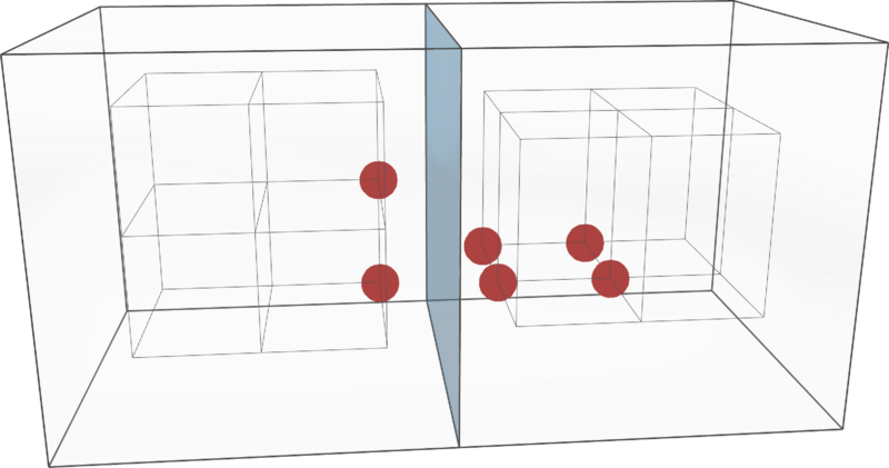
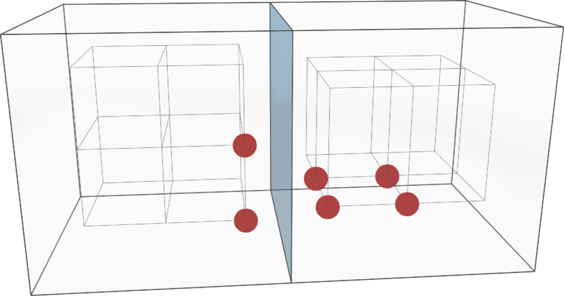
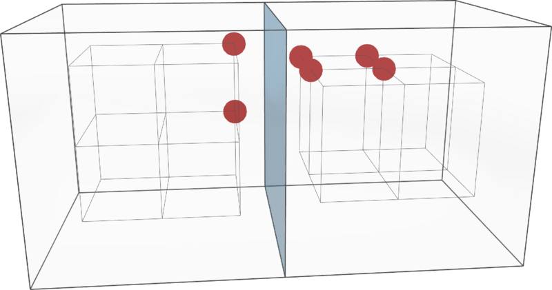
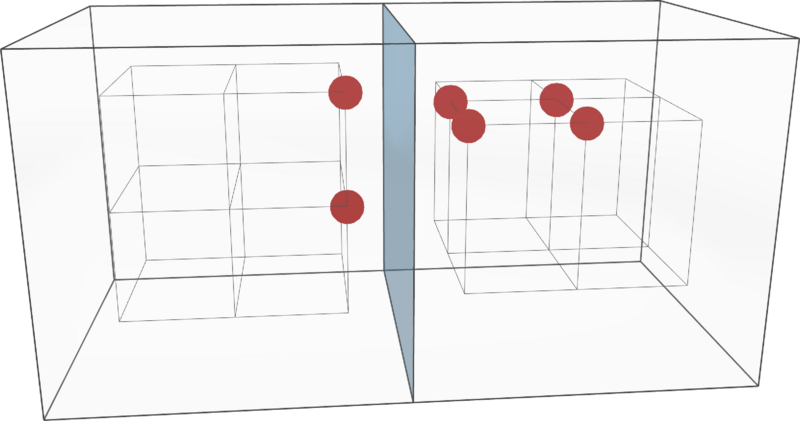
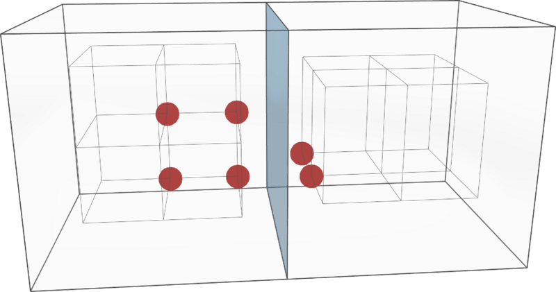
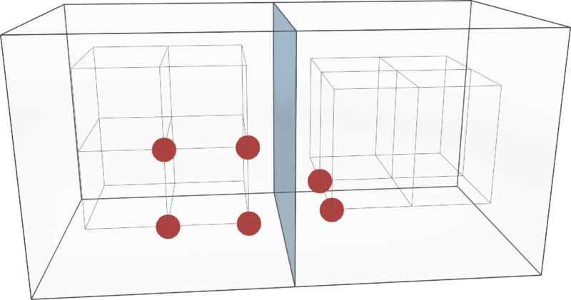
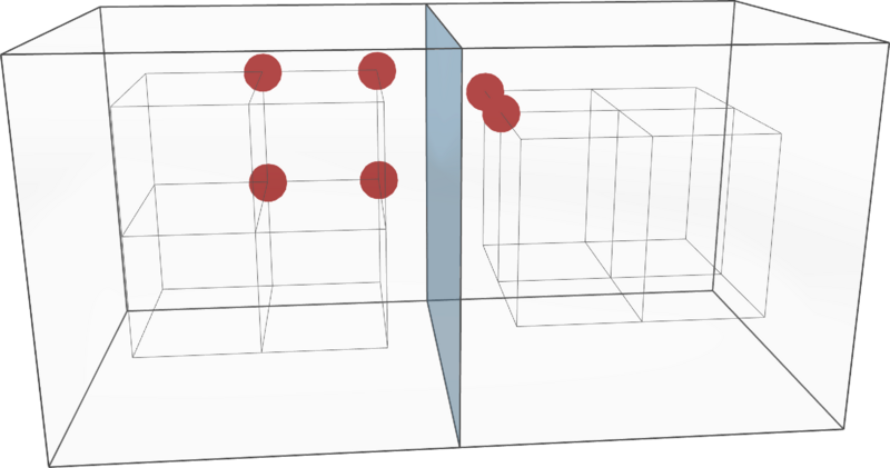
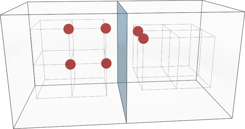
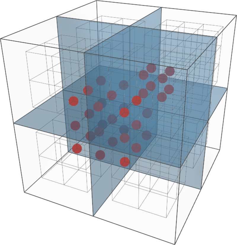
Figure 55: Examples of composite basis vectors on an edge adjacent to four hexahedron on a volumetric mesh. Three elements are quadratic and one is cubic. The continuity is everywhere. These -cell basis vectors are the volumetric analog to the two-dimensional vertex basis vector shown in figure 50b, one for each alignment index along the edge.
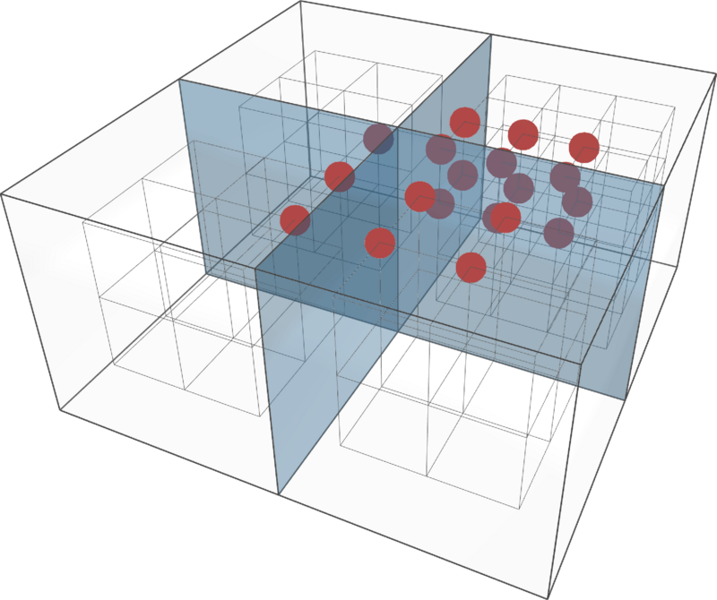
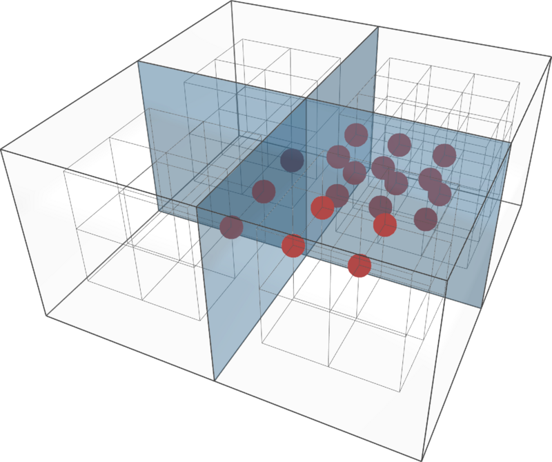
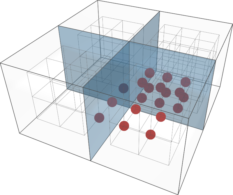
Figure 56a: Seven linear and one quadratic hexahedron meet at a regular vertex. The continuity is everywhere.
Figure 56b: Three linear and one quadratic hexahedron meet at an extraordinary vertex. The continuity is everywhere.
Figure 56: Several examples of composite vertex basis vectors on volumetric meshes. The degree and continuity for each example is indicated. Figure 56b is an example of an extraordinary vertex on a volumetric mesh, constructed by filling a tetrahedron with hexahedral cells. Figure 56c is analogous to the two-dimensional example in figure 50a. In figure 56d notice the far corner Bernstein index is missing on the cubic cell, analogous to the two-dimensional example in figure 50d.
5.2.6 Subordinate basis vectors
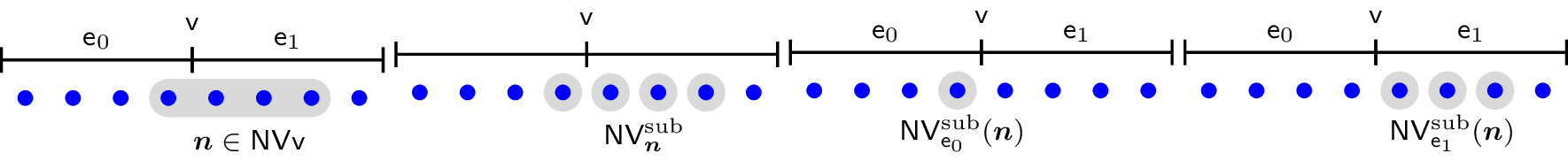
By definition, the constraint set for a -cell , , is a superset of the constraint set of any higher dimensional cell having in its boundary. Consequently, the basis vectors in can be expressed locally in terms of the basis vectors associated with the -cells having in their shared boundary. Given , we define the set of -cell basis vectors associated with as and say that the members of are subordinate basis vectors or basis vectors subordinate to . The subordinate basis vectors of a set of basis vectors is also defined as .
We also define the subset of basis vectors subordinate to that are also basis vectors on an adjacent cell as
An example of subordinate basis vectors in one dimension are shown in figure 57.
Figure 57: An example of subordinate basis vectors in one dimension. The set of subordinate basis vectors of is , and are the subsets of subordinate basis vectors associated with edges and , respectively.
5.2.7 Basis vector boundaries
The U-spline algorithm relies on relationships between basis vectors associated with adjacent topological features in order to construct basis vectors from the global set. These relationships are most conveniently expressed by introducing a notion of boundary to the mapped indices associated with nonzero entries in the basis vector.
It has been shown that basis vectors can be represented in terms of the basis vectors associated with higher-dimensional adjacent cells. Having constructed a basis vector, , for a -cell, , we loosely define the boundary with respect to an adjacent -cell, , as the most distant elements chosen from the set of subordinate basis vectors . We will denote this set by and make the definition more precise. We first give definitions for the three cases relevant to one and two dimensions and then define basis vector boundaries in arbitrary dimension.
5.2.7.1 Basis vector boundaries in one dimension
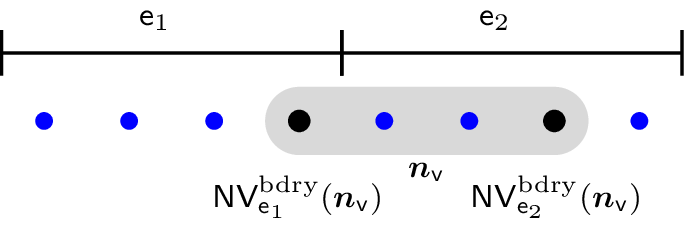
For the case of a basis vector associated with a vertex in the one-dimensional setting, we begin by defining an indexed submesh domain over the two edges adjacent to the vertex, such that the origin lies at the vertex, and the associated index mappings are for each edge . Then, the boundary with respect to the edge is given by where In figure 58 we see a basis vector on a vertex on a one-dimensional mesh. Associated with each adjacent edge and is a boundary set, and , which contains the subordinate basis vector that makes up the boundary in the direction of the respective edge. These are represented as black circles. The full set of boundaries is obtained by taking the union of all boundary sets generated by the edges adjacent to :
Figure 58: An example of basis vector boundaries on a vertex null vector on a one-dimensional mesh.
5.2.7.2 Basis vector boundaries in two dimensions
In a two-dimensional setting we must consider the boundaries of edge basis vectors and vertex basis vectors. The boundaries of edge basis vectors are constructed from the basis vectors of the adjacent face systems, which are just the standard Bernstein basis functions. Given an edge with basis vector adjacent to a face , the subordinate subset is and the associated index set is . We form the mapped points associated with and partition it with respect to the projection onto the edge : The boundary set is formed by taking the index associated with the most distant point in each equivalence class: Again, the full boundary is given by
The boundary set for a vertex basis vector in the two-dimensional setting is formed from the basis vectors associated with an edge adjacent to the vertex . The construction is similar to the construction presented for the boundary of edge basis vectors. We form the set containing the set of mapped index points for each vector in :
The chart is chosen so that both elements adjacent to the edge are mapped consistently and that lies at the origin. We partition the set of Greville point sets into equivalence classes with respect to the projection perpendicular to the edge and form the boundary set by taking the most distant element from each equivalence class. Given an equivalence class , we define the maximum of this equivalence class as the set of points whose projection onto the line in the direction of is greatest:
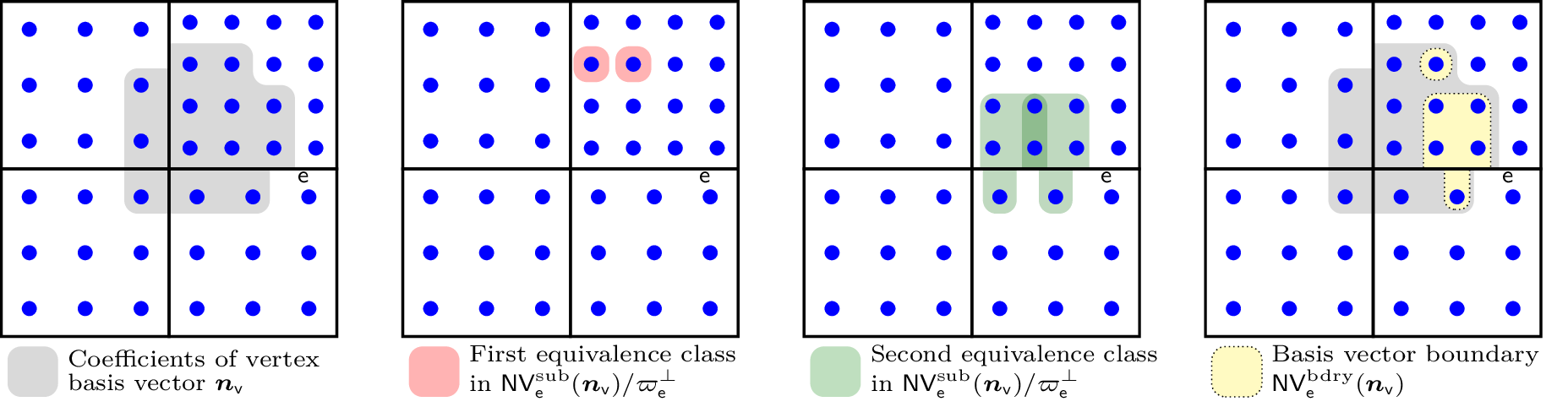
In figure 59 a vertex basis vector on a two-dimensional mesh with uniform degree is seen on the left. An equivalence class with respect to the projection perpendicular to the edge contains two subordinate basis vectors, as seen in the middle. The rightmost subordinate basis vector from the equivalence class makes up the basis vector boundary, as seen on the right. Similarly, in figure 60 on the left we see a vertex basis vector on a two-dimensional mesh with mixed degree. In this case there are two equivalence classes with respect to the projection perpendicular to the edge , each of which contain two subordinate basis vectors. The boundary set is made up of the rightmost subordinate basis vectors from each equivalence class, as seen on the right. The full boundary is once again obtained by uniting the boundary sets associated with every edge adjacent to
Figure 59: The boundary of a vertex basis vector on edge , on a quadratic mesh with continuity. In this case, there is only one equivalence class, which contains two subordinate basis vectors. The rightmost subordinate basis vector from the equivalence class makes up the basis vector boundary.
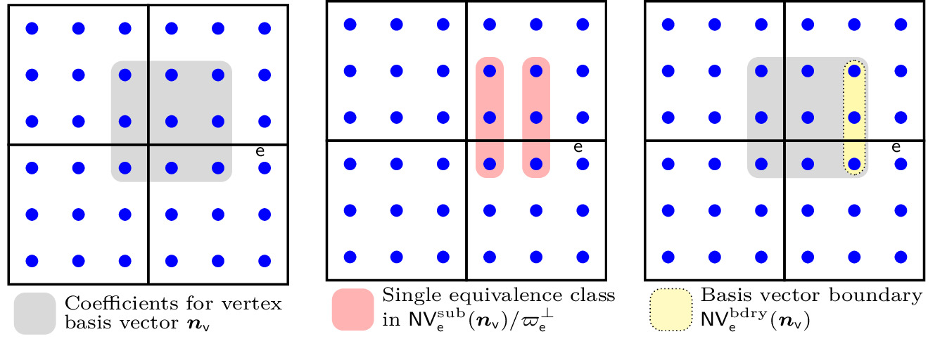
Figure 60: In the presence of local variation in degree, the boundary of a vertex basis vector on edge may be determined from more than one equivalence class. The rightmost subordinate basis vectors from each equivalence class make up the basis vector boundary. All the interfaces have continuity.
5.2.7.3 Basis vector boundaries in arbitrary dimensions
The boundary set for a -cell basis vector in the -dimensional setting is formed from the basis vectors associated with a -cell adjacent to , . The description for constructing the boundary set for a basis vector in arbitrary dimensions is a direct generalization of the description in Basis vector boundaries in two dimensions for vertex basis vectors in two dimensions, by taking equation , equation , equation , equation and replacing the vertex with and the edge with . In the general description, the chart is chosen so that all elements adjacent to are mapped consistently and that one of the vertices adjacent to lies at the origin.
5.3 Basis vectors in arbitrary dimensions
We describe how to build basis vectors on a -cell from a -dimensional Bézier mesh, . The description is recursive, and we begin with the base case: the basis vectors on a -cell are the Bernstein functions which span the Bernstein space assigned to the element. Then, the basis vectors on a -cell , are constructed as follows.
5.3.1 Composite cell basis vectors
Composite -cell basis vectors are formed from multiple adjacent -cell basis vectors. Each composite -cell basis vector is associated with a choice of inclusion distances (Inclusion distances) and alignment index (Alignment sets). An example of selecting a choice of inclusion distances is shown in figure 47.
We begin by placing indexed submesh domains denoted over each set of elements adjacent to each -cell adjacent to (with their origins set to ), and then partitioning the mapped index sets of the basis vectors associated with each -cell into equivalence classes with respect to the parallel equivalence relation on the -cell . We then identify the equivalence classes for which the minimum projection onto the -cell is less than or equal to : where is the parameter coordinate parallel to and perpendicular to . An example of these equivalence classes is shown in figure 48.
Let . ( is defined in Adjacencies. ) We form the sets containing all indices whose associated cell is adjacent to and whose associated submesh Greville point is a part of elements of We form the set of Greville points that are fixed points of the parallel projectors onto : We take all basis vectors whose projections onto the -cells perpendicular to lie in : In the case that then . In figure 49, we see an example of these basis vector subsets marked with dotted lines.
The set of indices associated with is The full set of indices associated with is Given an alignment index and a choice of , we can now define the index set for the composite -cell basis vector as
We consider all possible alignment indices and all possible values of on to construct the set of all composite -cell basis vectors. We use to represent this set. The full set of indices contained in this set is An example of a set of composite vertex basis vectors is shown in figure 50.
5.3.2 Simple cell basis vectors
Each simple -cell basis vector is formed from a single -cell basis vector on an adjacent -cell, one for each -cell basis vector whose index set is not subsumed by . We use to represent this set: An example of a set of simple vertex basis vectors is shown in figure 51.
5.3.3 The full set of cell basis vectors
The full set of -cell basis vectors is found by combining the set of composite -cell basis vectors with the set of simple -cell basis vectors: Once the index set for each -cell basis vector has been obtained, the constraint system can be solved to obtain the coefficient values and construct the basis vector.
5.4 The U-spline basis
Determine the index support for each -cell basis vector associated with each -cell (see Basis vectors for cell nullspaces).
Determine the index support of each U-spline basis vector by constructing a corresponding core graph (see The core graph).
Determine the basis vector of each U-spline basis function by solving the rank one null space problem (see The rank one null space problem).
Normalize the set of U-spline basis vectors to determine the set of U-spline basis functions (see Normalization).
5.4.1 The core graph
In order to construct U-spline basis vectors or, equivalently, U-spline basis functions, we need to create collections of vertex basis vectors and represent relationships between them. We do this by defining a core graph for each U-spline basis function. A core graph is a directed acyclic graph that combines adjacent vertex basis vectors into the index support for a single U-spline basis vector . An algorithm to compute is given in algorithm 1.
5.4.1.1 Cores
Each node in the graph, called a core and denoted by , corresponds to a set of vertex basis vectors, i.e., . To retrieve the core associated with a vertex we use . The boundary of a core in the direction of an edge , denoted by , is computed in the same manner as basis vector boundaries (Basis vector boundaries). The set of children cores of is denoted by . We say that cores and are conforming if on a shared edge . Edges between conforming cores represent parent/child relationships in .
5.4.1.2 Expansion edges
The core graph algorithm functions by iterating over candidate expansion edges on which to expand. An expansion edge is a directed edge from vertex to vertex , denoted . For the subsequent definitions it is convenient to define several auxiliary sets. The set of expanding basis vectors on a vertex adjacent to a core is given by The set of interacting edges is given by
The set of covered edges is given by Finally, let be the set of directed edges for which the algorithm has tried and failed to find a conforming child core. Then, the set of candidate expansion edges are given by: The core graph algorithm proceeds in a breadth-first manner. That is, in a graph with multiple candidate expansion edges, we prioritize those edges originating from cores closest to the root of the graph.
5.4.1.3 Algorithm
◾ Compute core graph from given vertex basis vector
1: procedure ComputeCoreGraph()
2: ▷ The root core consists of the input null vector.
3: ▷ Initialize the graph by inserting the root core.
4: while do▷ test comment
5: ▷ Get next expansion edge from .
6: if is an ancestor of then▷ A connection from to would create a cycle.
7: ▷ Mark as failed and go to next iteration.
8: continue
9: end if
10: ▷ Construct a new core on that conforms to .
11: if then▷ If is empty, expansion failed along this edge.
12:
13: continue
14: end if
15: ▷ Merge with any existing null vectors in .
16: ▷ Add a graph edge from to .
17: for each do▷ Prune any children of that no longer conform.
18: if then
19: remove and all descendants from
20: end if
21: end for each
22: ▷ Remove and its opposite from failed edges.
23: end while
24: ▷ The algorithm succeeds only if it terminates with no failed edges.
25: return , ▷ test return endline comment
26: end procedureAlgorithm 1: Compute core graph from given vertex basis vector
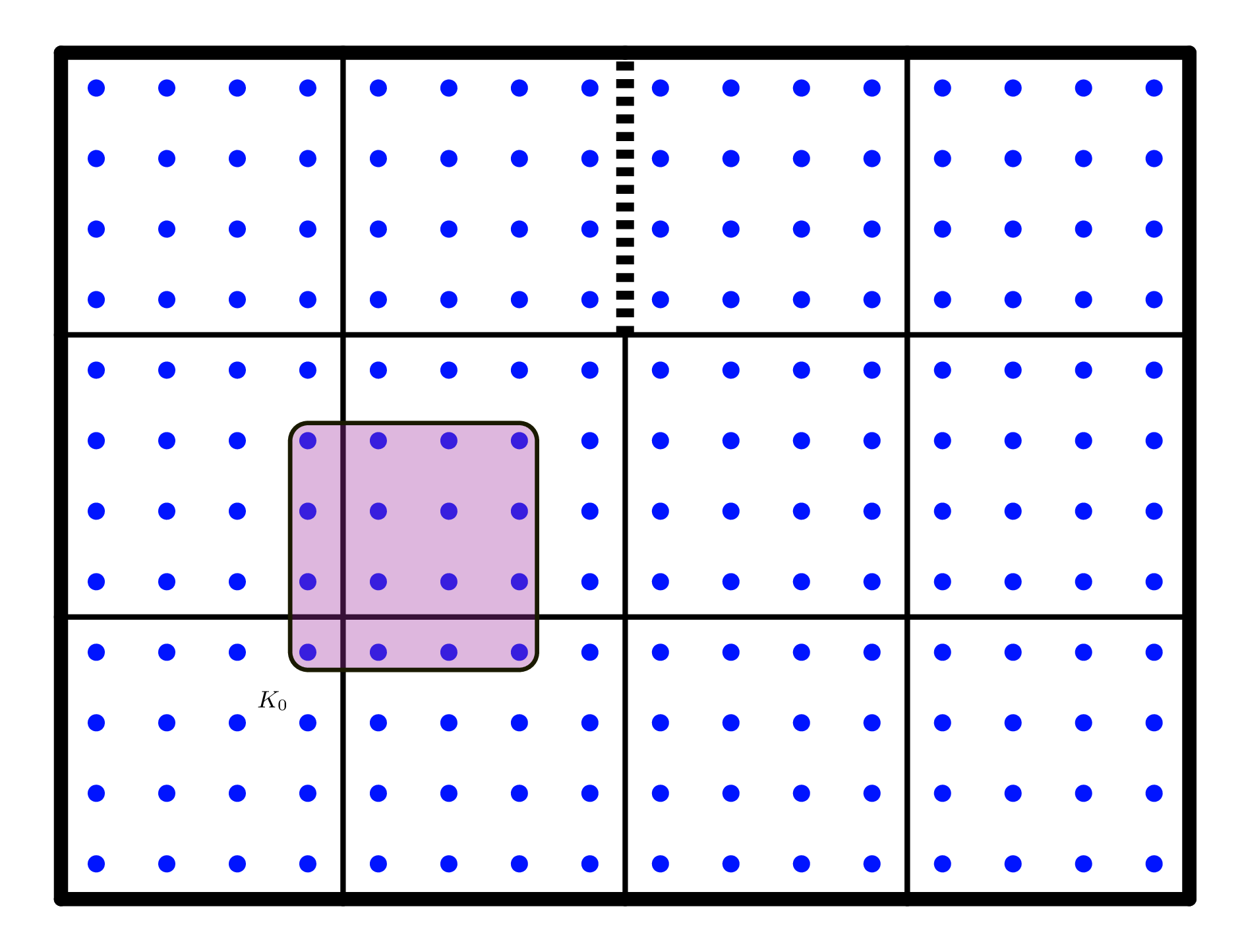
Algorithm 1 describes the procedure for constructing a core graph. To illustrate the behavior of the core graph algorithm, first consider the one-dimensional cubic U-spline mesh shown in figure 61, where each feature of a core graph is depicted, including the root core , two child cores and , and the expansion candidate edges which resulted in the two children being added to the graph. Next, consider the two-dimensional cubic U-spline mesh shown in figure 62. This mesh has twelve cells and continuity everywhere except for one edge which is , forming a supersmooth interface.
Figure 61: An example of a simple core graph on a one-dimensional cubic U-spline mesh. The continuity on the interfaces is .
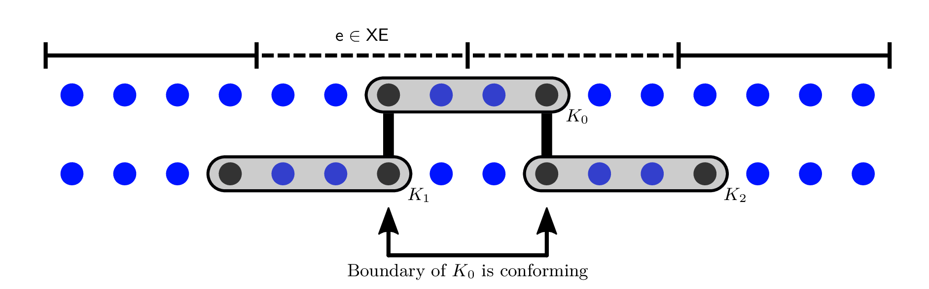
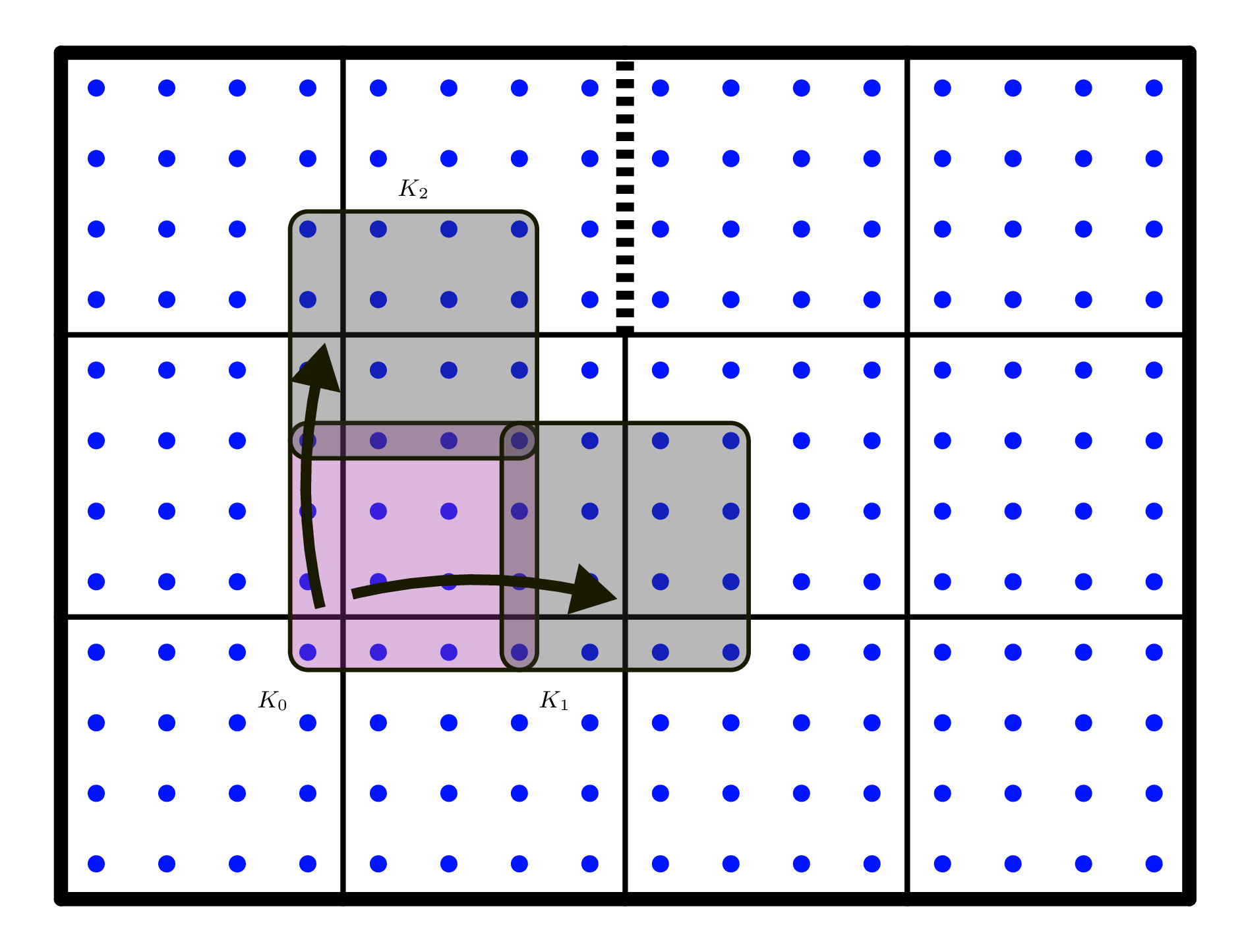
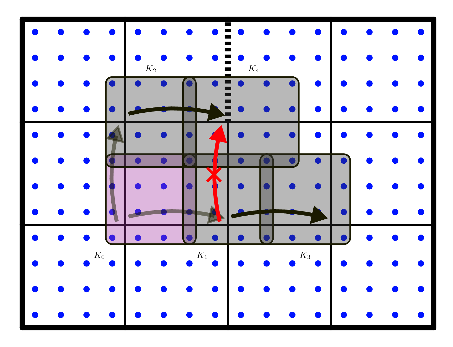
Figure 62c: The core graph is expanded a second time, to the right on both legs of the graph, forming cores and . A failed expansion is encountered when trying to expand upwards from .
Figure 62: A two-dimensional core graph example. In this example, the U-spline mesh is a -by- bicubic mesh with a single supersmooth interface. All interior edges have continuity (thin solid lines) except for one, which has continuity (thick dashed line), forming a supersmooth interface.
5.4.2 The rank one null space problem
The U-spline index support is extracted from the combined index supports of the cores in . We then consider a restricted rank one constraint matrix and associated null space problem. In the multi-dimensional setting, the smoothness constraints often form a system of linearly dependent equations. That is, the constraint matrix is often not square, with the number of rows being greater than the number of columns . To solve for the Bernstein coefficients of the U-spline basis vector , one approach is to solve for the reduced row echelon form of via Gaussian elimination, resulting in a matrix with rows equal to . However, it has been shown that Gaussian elimination on floating point numbers leads to unacceptably high accumulated error when analyzing the null space of spline constraint equations [3].
An alternative approach is to cast the problem as the linear program Note that we have enforced the lower bound to preclude the trivial solution of . This linear program can then be solved using any number of established methods such as simplex methods or interior-point methods. We have used the revised simplex method implemented in the lp_solve package [13]. Thus far we have found this approach to be sufficient for solving our problems of interest, and as such have not compared the various algorithms that may be used to solve the above linear program. Instead, a detailed comparison of the solution methods that may be employed to solve the linear system of constraint equations for a given function will be the topic of a future work.
5.4.3 Normalization
To recover a partition of unity in the U-spline basis we perform a normalization step. In other words, we want to find a set of positive coefficients , such that where is a normalized U-spline basis function. This normalization is always possible due to the underlying structure of the null space .
This problem can be solved in a variety of ways such as by constructing a full rank linear system by sampling the U-spline basis at unique locations or by recasting the problem as a linear programming problem and solving it using a simplex method or similar technique as described in The rank one null space problem.
Note that there exists a set of non-negative coefficients, , such that This can be shown using the following reasoning. Since the function is an analytic function and for every we know that . This means there exists a set of coefficients, , such that Since by construction , where is the non-negative orthant, and is a polyhedral cone then is a polyhedral cone as well. This means that, in fact, the coefficients are also non-negative, i.e., . Consequently, we have that
5.5 Verification of U-spline space
The approach to building a basis on a U-spline mesh presented in The U-spline basis is algorithmic in nature. In order to verify that this algorithm will always successfully build a valid U-spline basis with the desired properties on every U-spline mesh, we performed extensive testing by running the U-spline algorithm on a large number and variety of one- and two-dimensional input U-spline meshes. For three-dimensional meshes, due to computational speed limitations we focused our testing on a specific set of tailor-made volumetric meshes that specifically conform to or violate each admissibility condition. A formal proof of the correctness of the algorithm is beyond the scope of this work.
The set of all admissible U-spline meshes is very large, and it is impractical to test every possible mesh configuration. In order to ensure that our test suite contained sufficient variety to provide reasonable evidence of the validity of the U-spline algorithm, for one- and two-dimensional meshes we leveraged the U-spline mesh classification system presented in Classification to generate test meshes within several of these classes, representing increasing levels of complexity.
5.5.1 Overview of verification procedure
We first generated meshes within the most structured class , and then proceeded to remove structure until finally a large number of meshes in the class were tested (see table 2 for a definition of each superscript). In one dimension, we focused on class . For each mesh, we used the U-spline algorithm to construct a set of basis functions. These basis functions were then analyzed to ensure they satisfied all the mathematical properties of a U-spline space as described in Mathematical Properties.
5.5.1.1 One dimension
For one-dimensional meshes, the class was selected, which allows any degree on each cell and continuity on each interface up to . This is the most unstructured class possible in one dimension.
5.5.1.2 Two dimensions
On two-dimensional meshes, five gradations of structure were selected.
: Tensor-product topology; degree and continuity propagate globally.
: Tensor-product topology; degree propagates globally but continuity may vary locally (including supersmooth interfaces).
: Tensor-product topology; continuity propagates globally but degree may vary locally.
: Meshes may include extraordinary vertices and triangles; degree propagates globally but continuity may vary locally.
: Fully unstructured.
Within each class, meshes were randomly constructed to include as much variation as possible while still conforming to the admissibility conditions described in Admissible Layouts. This included degree up to and continuity up to or when permitted, supersmooth continuity. The process of constructing these meshes involved starting with a specific base topology, listed below, and then applying further modifications as the class allowed, such as adding extraordinary vertices, triangles, and variations in degree and continuity. The base topologies used are as follows. Simple representations of these base topologies are shown in figure 63.
Line. A line topology is a non-periodic one-dimensional sequence of edges, and is denoted by .
Loop (has periodicity). A loop topology is a periodic one-dimensional sequence of edges, and is denoted by .
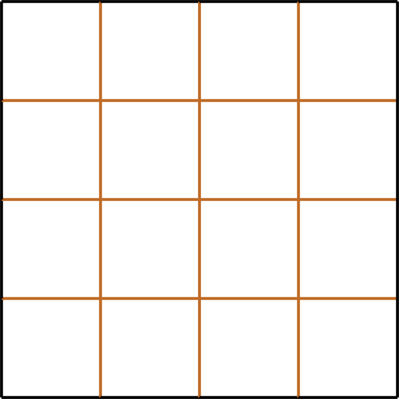
Regular grid. A regular grid topology is a tensor product of two non-periodic one-dimensional mesh topologies, and is denoted
Annulus (periodicity in one tensor product direction). An annulus topology is the tensor product of a periodic one-dimensional topology with a non-periodic one-dimensional topology, and is denoted
Torus (periodicity in both tensor product directions). A torus topology is the tensor product of two periodic one-dimensional topologies, and is denoted
Triangle. A triangle mesh topology is an unstructured mesh containing only triangles, and is denoted .
Mixed grid. A mixed grid mesh is a mesh containing both quadrilateral and triangular cells that is constructed by taking a tensor product mesh (grid, annulus, or torus), and then splitting a subset of the quadrilateral cells into two or more triangles. A mixed grid mesh is denoted .
Multi-patch. A multi-patch topology is constructed of multiple regular grid, mixed grid, or triangle meshes, sewn together along conforming boundaries. A multi-patch topology is denoted .
Following these guidelines, twenty-five thousand two-dimensional admissible U-spline meshes were constructed, with variation in degree, continuity, mesh size, and topology. In addition, several thousand one-dimensional admissible U-spline meshes of all combinations of degree and continuity were also constructed. The U-spline algorithm successfully constructed a basis on each of these meshes that was verified to satisfy all the mathematical properties of a U-spline space described in Mathematical Properties.
Figure 63: The three base tensor-product topologies used for constructing two-dimensional U-spline test meshes for verification.
5.5.1.3 Three dimensions
Due to computational speed limitations, it was impractical to generate and test volumetric meshes in the same way as was done in one and two dimensions. Instead, a specific set of tailor-made volumetric meshes were created that specifically conform to or violate each admissibility condition. Our tests demonstrated that the U-spline algorithm successfully built a valid U-spline basis with the desired properties on each of the admissible meshes.
5.6 U-spline test cases with Bézier extraction coefficients
5.6.1 U-spline extraction coefficients near a supersmooth interface
Figure 64: A four-by-three cubic U-spline mesh with continuity on all interior edges except for one which has continuity, forming a supersmooth interface. The Bernstein coefficients of the highlighted basis function are listed in table 4.
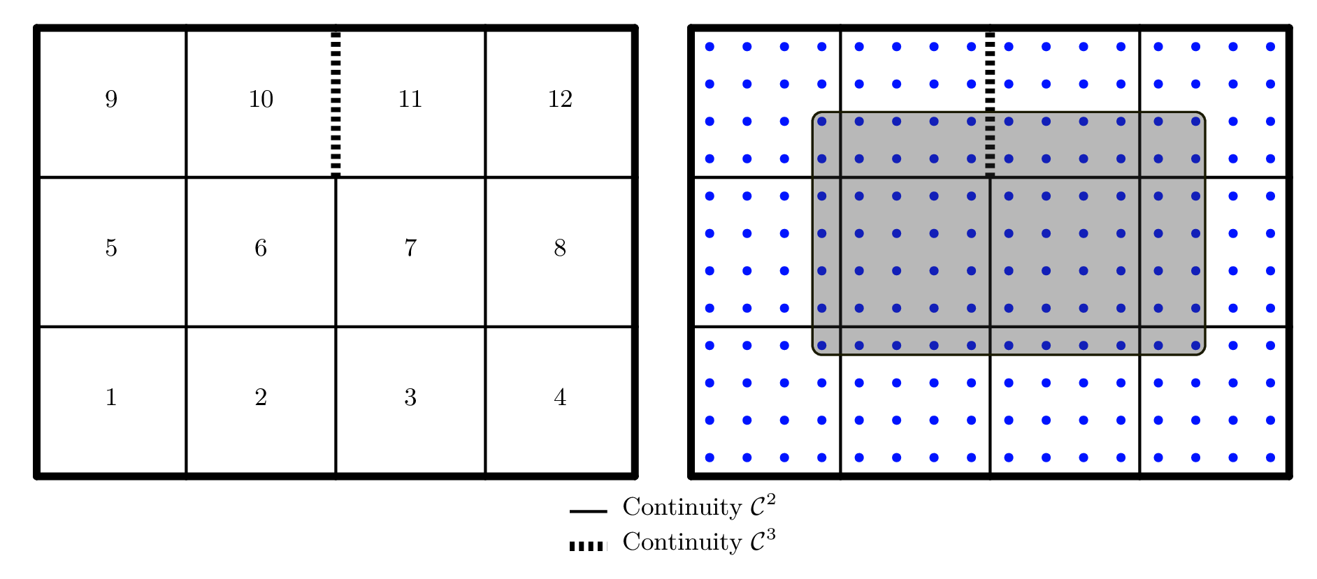
Table 4: The values of the nonzero Bernstein coefficients of the U-spline basis function highlighted in figure 64.
5.6.2 U-spline extraction coefficients with non-rectangular support
Figure 65: An example of a U-spline basis function that has a non-rectangular shape due to the close proximity of two continuity transitions near supersmooth interfaces. Notice the two perpendicular transition ribbons, starting at the vertices adjacent to the supersmooth interfaces, which touch at a common endpoint. This is an example of a basis function which is not possible with T-splines, which require basis functions to have a tensor product structure. The Bernstein coefficients of the highlighted basis function are listed in table 5.
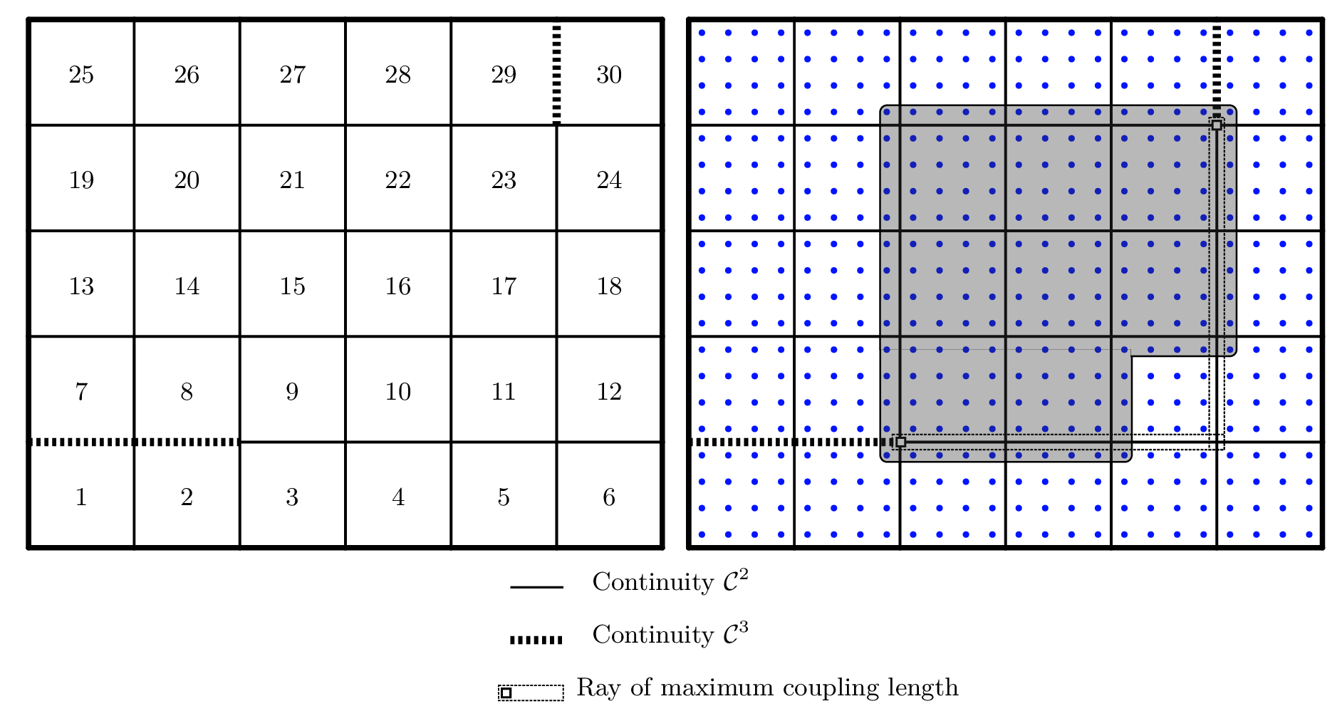
Figure 66a: The control points for a linear parameterization of the mesh in figure 65. The highlighted control point corresponds to the highlighted basis function.
Figure 66b: Contour plot of the basis function whose nonzero Bernstein coefficients are highlighted in figure 65.
Figure 66: Control points and basis function contours for the U-spline in figure 65.
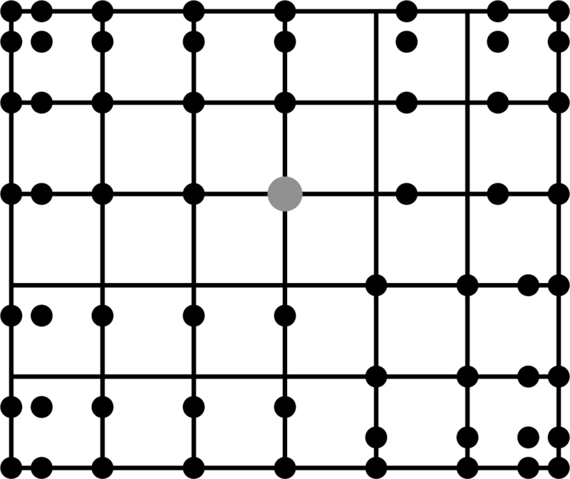
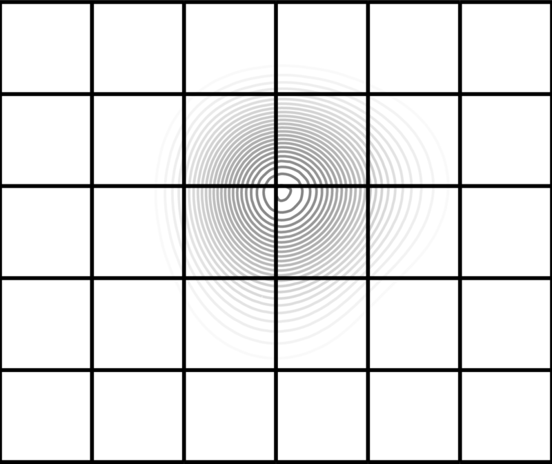
Table 5: The values of the nonzero Bernstein coefficients of the U-spline basis function highlighted in figure 65.
5.6.3 U-spline extraction coefficients on mesh equivalent to analysis-suitable T-spline with non-crossing edge extensions
Figure 67: Basis function on a U-spline that is equivalent to an analysis-suitable T-spline [56, 88]. The T-mesh of the equivalent T-spline is shown in figure 69. Note that the ribbons of maximum coupling length in this example are analogous to the non-crossing T-junction extensions which guarantee an analysis-suitable T-spline. The Bernstein coefficients of the highlighted basis function are listed in table 6.
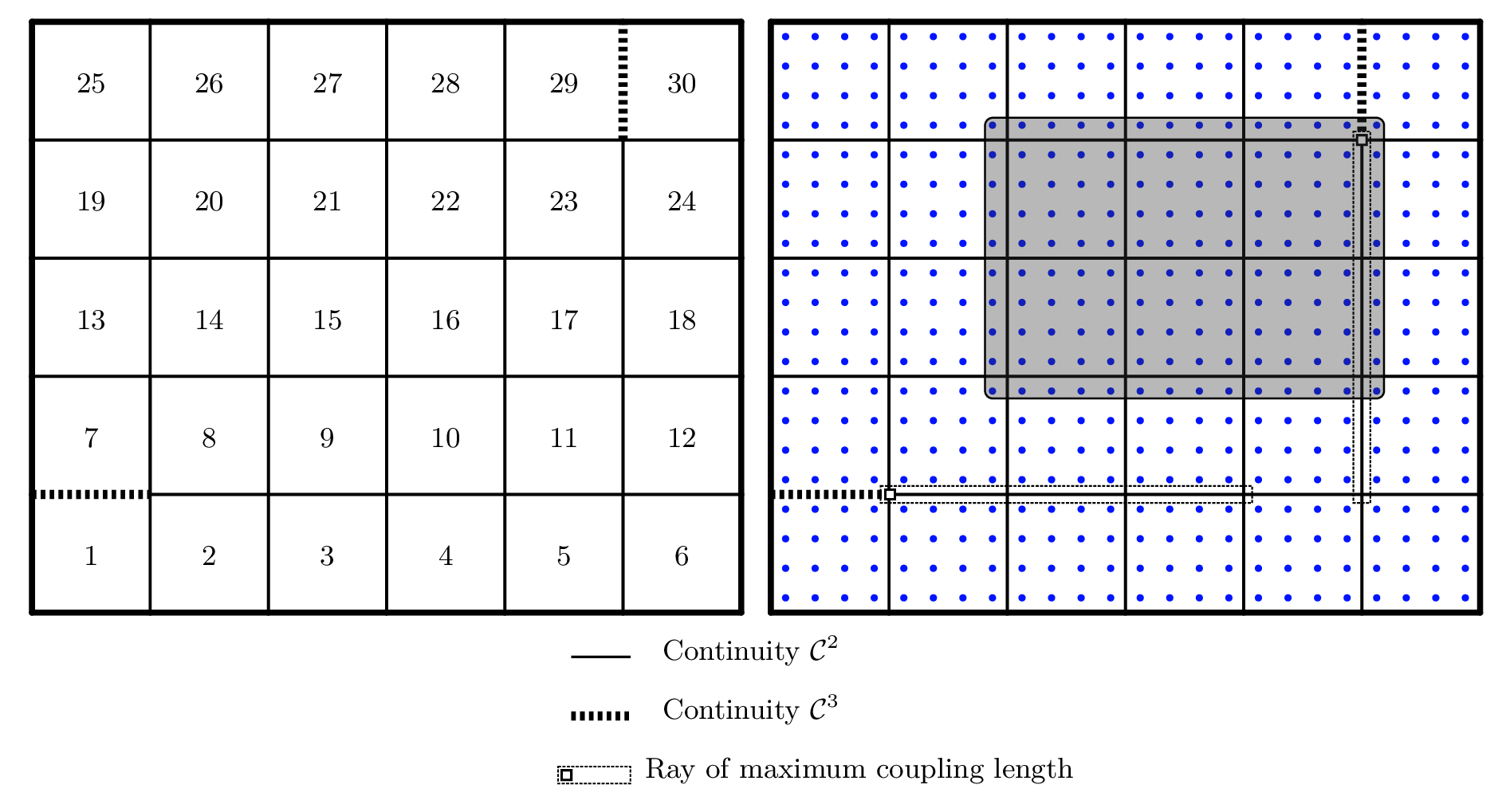
Figure 68a: The control points for a linear parameterization of the mesh in figure 67. The highlighted control point corresponds to the highlighted basis function.
Figure 68b: Contour plot of the basis function whose nonzero Bernstein coefficients are highlighted in figure 67.
Figure 68: Control points and basis function contours for the U-spline in figure 67.
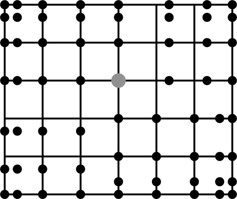
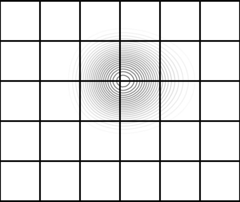
Figure 69: The T-mesh for a cubic T-spline which is equivalent to the U-spline mesh in figure 67 [88]. The area highlighted in yellow corresponds to the Bézier elements of the U-spline mesh. The dotted lines next to the T-junctions are the lines of reduced continuity, where there is still continuity [85]. It is notable to observe that the vertices associated with the T-junctions on the T-mesh are not the same as the vertices adjacent to the supersmooth interfaces on the U-spline mesh, due to the lines of reduced continuity.
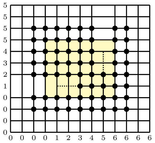
Table 6: The values of the nonzero Bernstein coefficients of the U-spline basis function highlighted in figure 67.
5.6.4 U-spline extraction coefficients near an extraordinary vertex
Figure 70: The support of one of the basis functions on a cubic mesh with a valence- extraordinary vertex. The edges about the extraordinary vertex are creased in a stair-step pattern, starting at and incrementally increasing continuity until . The Bernstein coefficients of the highlighted basis function are listed in table 7.
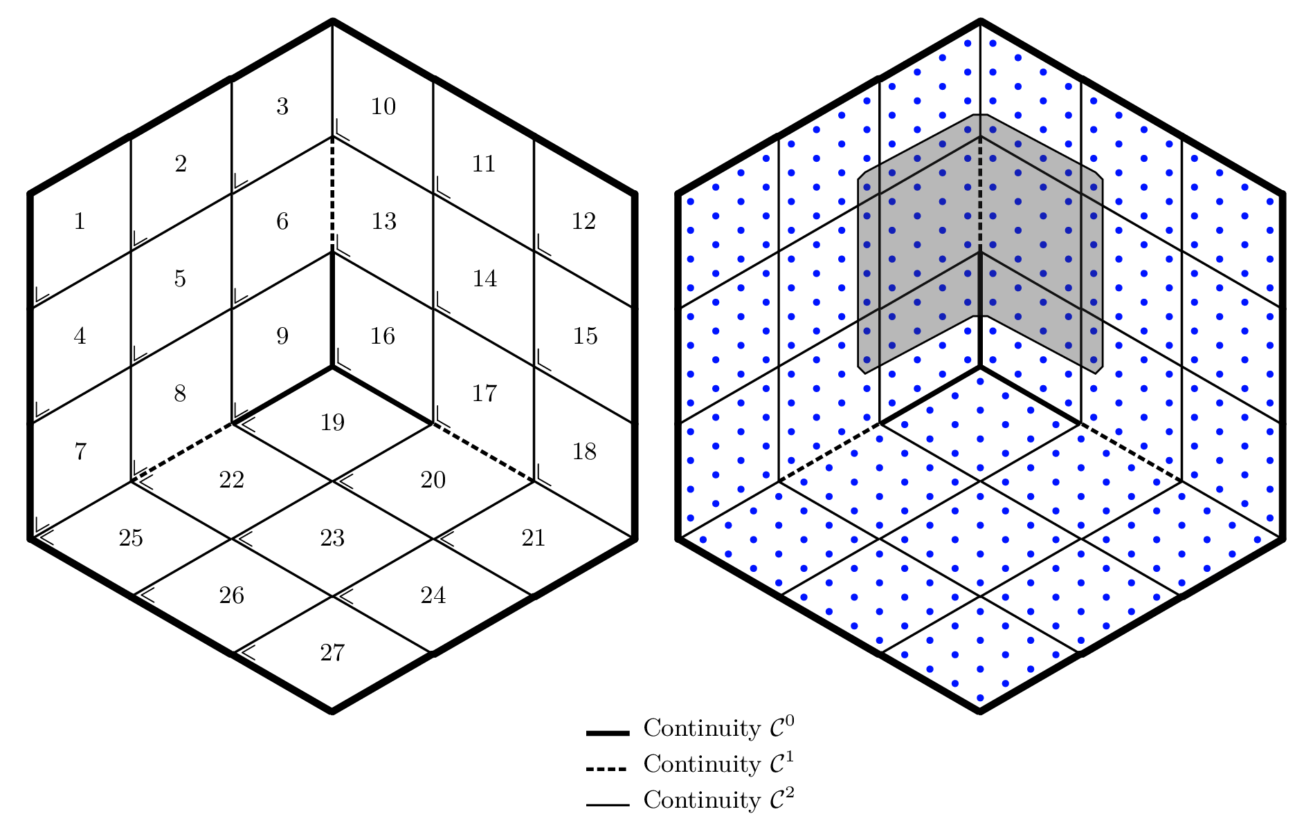
Figure 71a: The control points for a linear parameterization of the mesh in figure 70. The highlighted control point corresponds to the highlighted basis function.
Figure 71b: Contour plot of the basis function whose nonzero Bernstein coefficients are highlighted in figure 70.
Figure 71: Control points and basis function contours for the U-spline in figure 70.
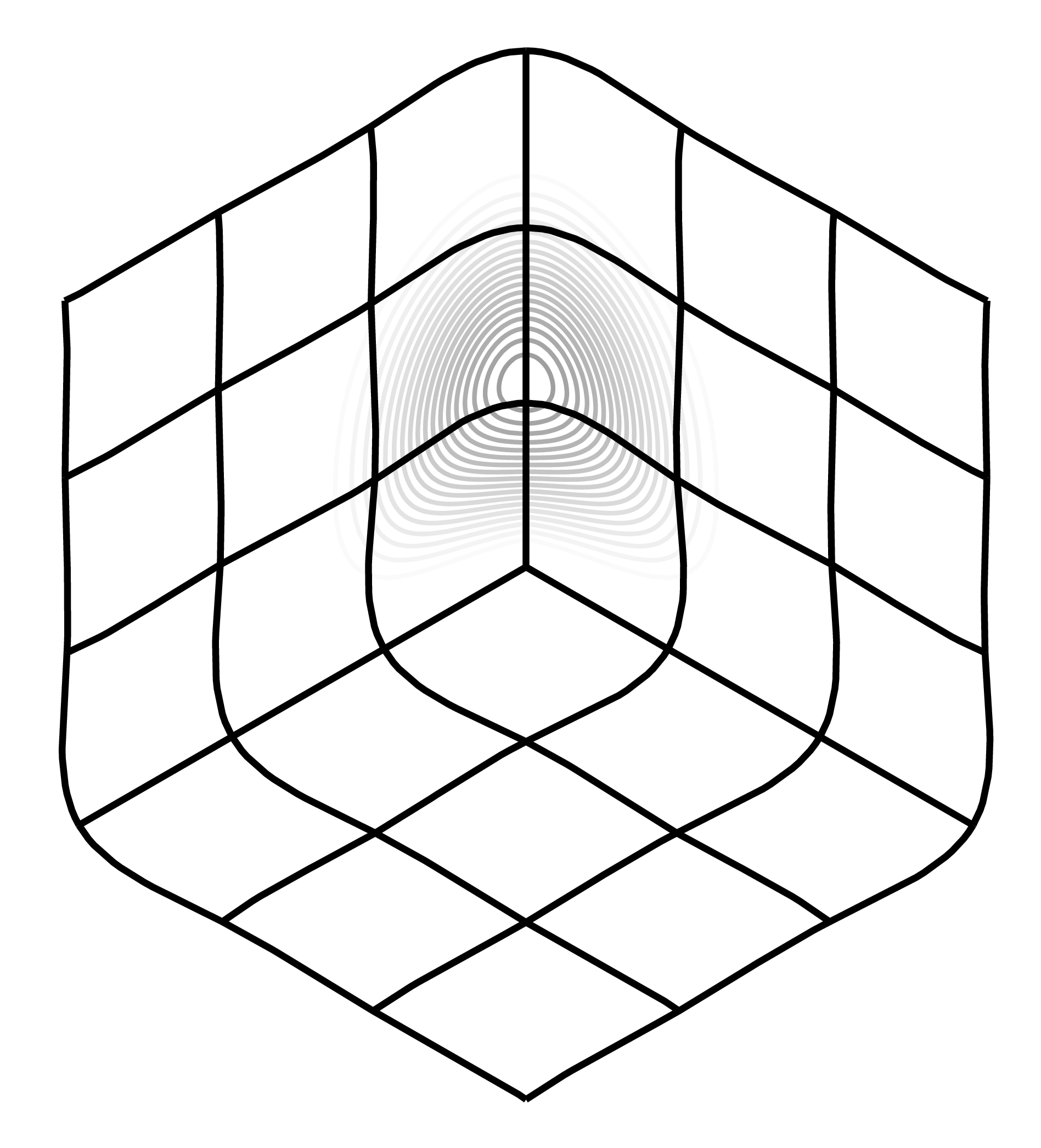
Table 7: The values of the nonzero Bernstein coefficients of the U-spline basis function highlighted in figure 70.
5.6.5 U-spline extraction coefficients near a triangle
Figure 72: The support of basis functions on a mesh that includes triangles. The values of the control points of the highlighted functions are listed in table 8 and table 9.
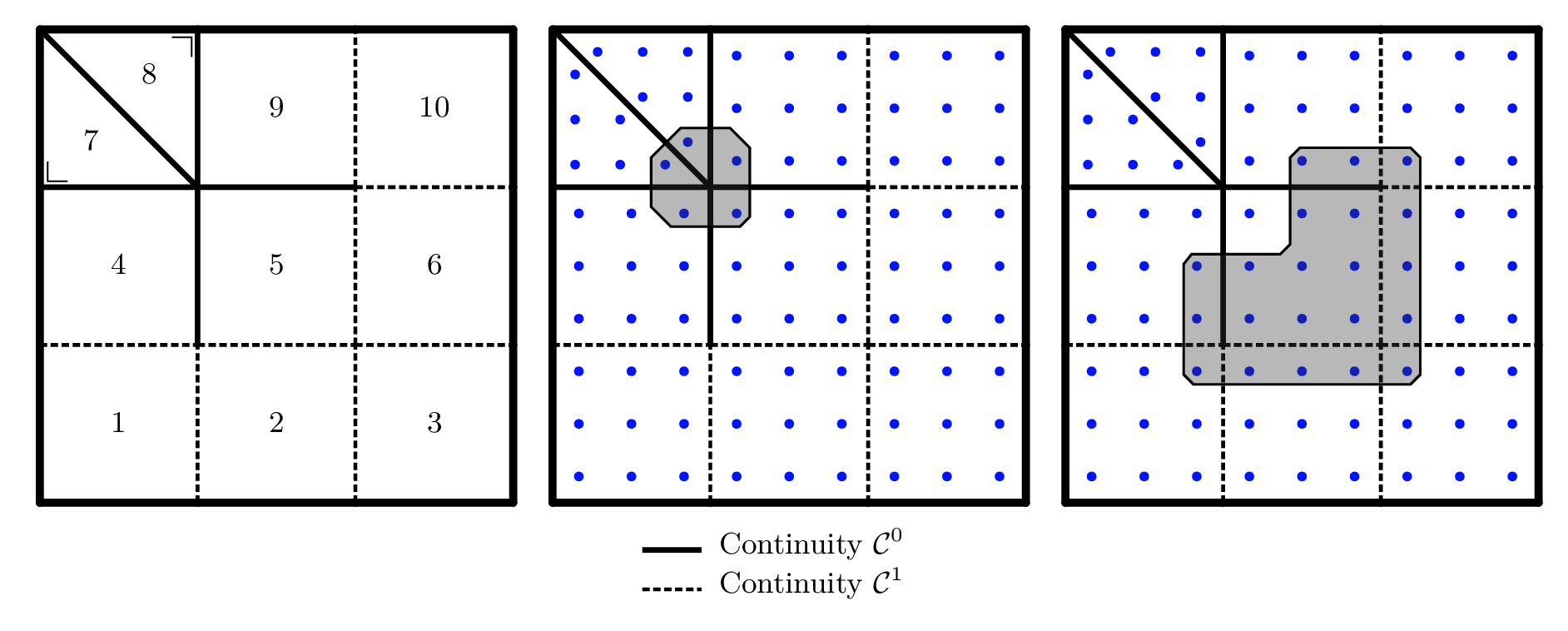
Figure 73a: The control points for a linear parameterization of the mesh in figure 72. The highlighted control point corresponds to the left highlighted basis function.
Figure 73b: Contour plot of the basis function whose nonzero Bernstein coefficients are highlighted on the left in figure 72.
Figure 73: Control points and basis function contours for the U-spline basis function highlighted on the left in figure 72.
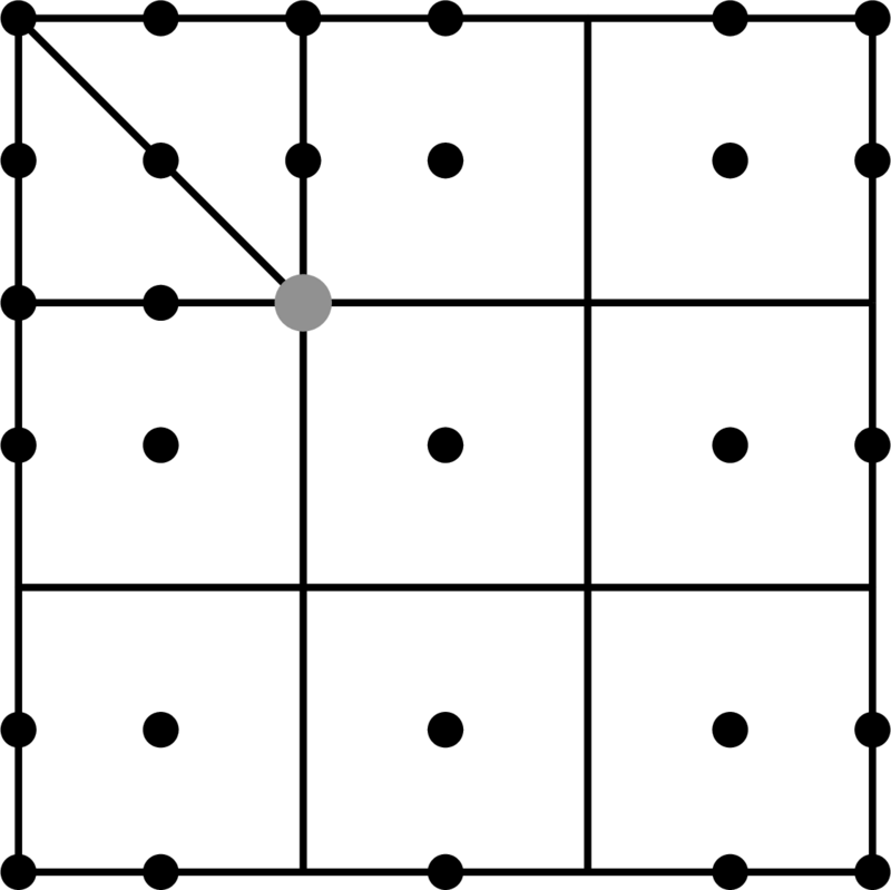
Figure 74a: The control points for a linear parameterization of the mesh in figure 72. The highlighted control point corresponds to the right highlighted basis function.
Figure 74b: Contour plot of the basis function whose nonzero Bernstein coefficients are highlighted on the right in figure 72.
Figure 74: Control points and basis function contours for the U-spline basis function highlighted on the right in figure 72.
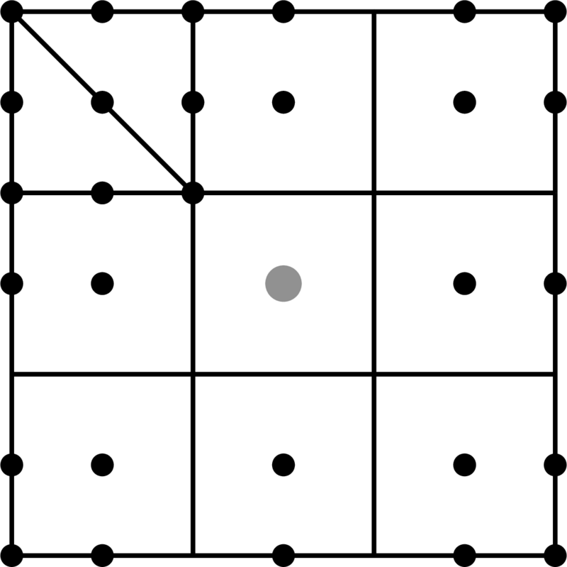
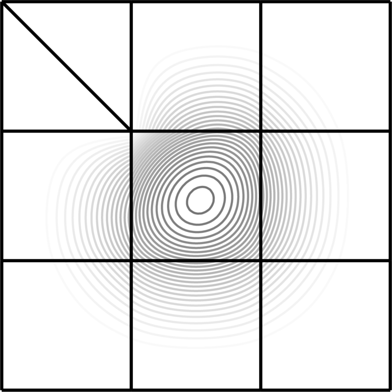
Table 8: The values of the nonzero Bernstein coefficients of the U-spline basis function highlighted in figure 72 on the left.
Table 9: The values of the nonzero Bernstein coefficients of the U-spline basis function highlighted in figure 72 on the right.
5.7 Ribbon processing
A ribbon of maximum coupling length is constructed on a mesh beginning at an origin -cell adjacent to an initial Bernstein coefficient, and then adding interfaces one by one beginning at the origin -cell to form the tail . We use to represent the number of interfaces present in the tail . As shown in figure 75 and figure 76, to determine the length of the tail (or coupling distance) we process a sequence of connected interfaces where the continuity assigned to each traversed -cell is set to and the degree of each traversed interface is set to .
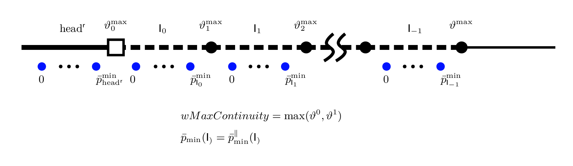
Conceptually, this process extracts a one-dimensional U-spline mesh (where the vertices and edges of the one-dimensional mesh correspond to the -cells and interfaces of the parent mesh), and determines how far the specified Bernstein coefficient couples with the neighboring coefficients assigned to the edges in the one-dimensional mesh given the continuity constraints assigned to each vertex. algorithm 2 describes the procedure used to determine the edges in the ribbon tail leveraging the notation introduced in figure 75 and figure 76. The input parameters of the procedure include the interface at the head of the ribbon , the origin vertex , and is the index of the initial Bernstein coefficient in . Several examples of ribbons of maximum coupling length are shown in figure 77.
A ribbon of length is said to be truncated if and the value of the Bernstein index computed for the final interface is greater than zero, as shown in algorithm 2. The bottom two examples in figure 77 show truncated ribbons.
See Building intuition: The U-spline mesh for an intuitive example of constructing a ribbon of maximum coupling length.
Figure 75: The features of a ribbon of maximum coupling length on a two-dimensional U-spline mesh. The perpendicular interfaces on the th vertex are assigned continuities and .
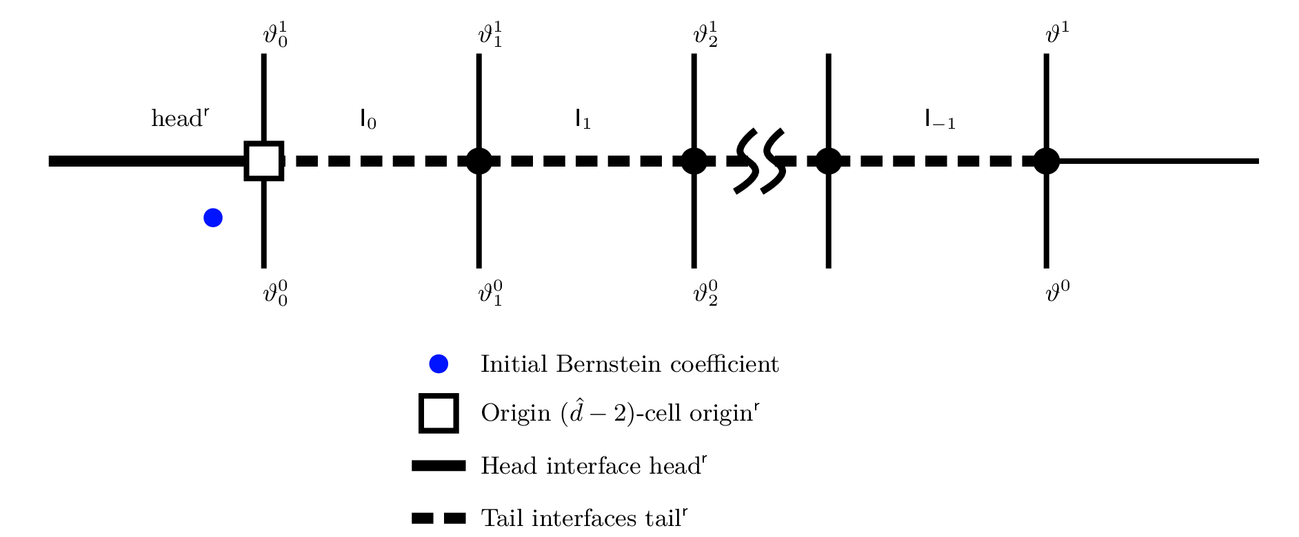
Figure 76: A ribbon that has been collapsed into a one-dimensional U-spline mesh. The continuity assigned to each vertex is the maximum of the perpendicular interfaces in the two-dimensional mesh. The degree of each one-dimensional cell is the minimum of the parallel degrees of the adjoining cells from the two-dimensional mesh, in the direction parallel to the ribbon. The Bernstein coefficients are labeled as they are indexed in algorithm 2.
◾ Build ribbon of maximum coupling length
1: procedure ComputeRibbon()▷
2: ▷ The array that will contain the interfaces in the tail.
3: ▷ Counter for the length of the tail.
4: ▷ If the ribbon is found to be truncated, this will be set to true later.
5: ▷ The Bernstein index counter used to determine the length of the ribbon.
6: ▷ The index used in the loop to reference the head interface.
7: ▷ The index used in the loop to reference the origin -cell.
8: //Loop until the maximum coupling length is reached.
9: loop
10: ▷ Save the Bernstein index on interface for later reference.
11: //Get the max smoothness on the interfaces perpendicular to the ribbon on .
12: ▷ In other words, .
13: ▷ Get the min parallel degree on the previous interface.
14: ▷ We compute the Bernstein index for interface .
15: if then
16: ▷ If the Bernstein index for is valid, then we add to the tail.
17: ▷ Increment the number of interfaces in the tail.
18: else
19: //Here, refers to the value of on , the final interface of the tail .
20: if then
21: //Since , the only way on interface to be less than is for the final interface to have reduced continuity.
22:
23: end if
24: break▷ Break out of the loop.
25: end if
26: end loop
27: ▷ Assemble the ribbon.
28: return ▷ Return the result.
29: end procedureAlgorithm 2: Build a ribbon of maximum coupling length, starting at head interface , origin -cell , and initial Bernstein index (see figure 75 and figure 76 for notation).
Figure 77: Several examples of the construction of ribbons of maximum coupling length. The Bernstein index marked by a hollow circle in each cell is the index referenced by in each loop of algorithm 2. Note that the bottom two ribbons are truncated.
5.8 Interface Continuity Constraints in Two Dimensions
We now consider constructing constraints on the interface between two cells on a two-dimensional U-spline mesh. We consider three cases: (1) the interface between two quadrilateral cells, (2) the interface between a quadrilateral and triangle cell, and (3) the interface between between two triangle cells. Without loss of generality, in each case we express these constraints with respect to the interface-aligned parameterizations indicated by the axes in figure 78, figure 79, and figure 80. We recognize that in practice, arbitrary relative rotations of the parameterizations on the adjacent cells must be accounted for, but for simplicity of exposition we assume the adjacent cells have the aligned coordinate systems as indicated.
We also assume the existence of a degree-elevation operator that maps the coefficients of a Bernstein polynomial of degree to a new vector of coefficients of a Bernstein polynomial of degree , thus representing the original function with a new basis of degree . Thus,
where the nonzero entries of the matrix operator are given by
5.8.1 Quadrilateral-Quadrilateral Interface
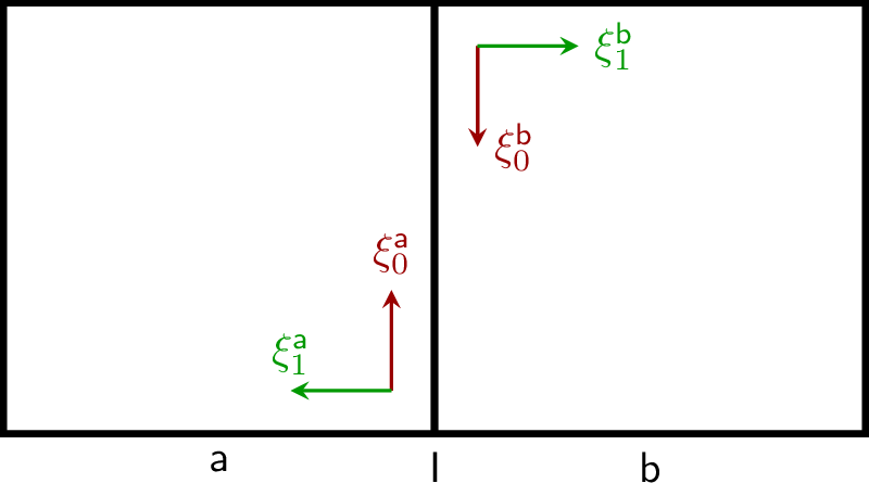
Consider two quadrilateral cells and on a two-dimensional mesh, separated by interface as shown in figure 78. Each cell has been assigned a box-like parameterization with parent coordinates . These cells have their parameterizations oriented such that the parameters on cell and the parameter on cell each point parallel the interface (although in opposite directions). Let parameterize the shared interface , and be defined as . The lengths of the parametric domain on cell are , and the lengths of the parametric domain on cell are . The mapping from the parent to the parametric domain in each parametric direction on each cell is . The degree assigned to cell is , and the degree assigned to cell is .
Figure 78: Two cells separated by interface on a two-dimensional mesh. We consider building the continuity constraint on the derivative of order on this interface.
A piecewise polynomial with support over and can be written in Bernstein form as
We can write the continuity constraint on the derivative of order across the interface as and if we can enforce the above equality constraint by instead enforcing In the case that , we define . The degree-elevation operator is used here to map the respective Bernstein coefficents to a degree Bernstein space on the shared interface. Substituting in and rearranging yields the constraints in homogeneous form
An example of the nonzero constraint equation coefficients on an interface between two quadrilaterals of degree and may be seen in figure #f, with the full constraint matrix listed in equation .
5.8.2 Quadrilateral-Triangle Interface
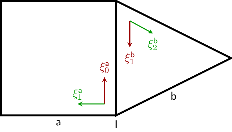
Consider a quadrilateral cell and a triangle cell on a two-dimensional mesh, separated by interface as shown in figure 79. The quadrilateral cell has been assigned a box-like parameterization with parent coordinates , and the triangle cell has been assigned a barycentric parameterization with parent coordinates . These cells have their parameterizations oriented such that the parameter on the quadrilateral and the parameter on the triangle each point parallel the interface (although in opposite directions). Let parameterize the shared interface , and be defined as .
The degree assigned to cell is , and the degree assigned to cell is . All barycentric index tuples in the triangle cell are expressed with two indices and corresponding to barycentric coordinates and . The remaining index corresponding to is omitted, but is implicitly defined to be equal to .
Figure 79: A quadrilateral cell and a triangle cell separated by interface on a two-dimensional mesh. We consider building the continuity constraint on the derivative of order on this interface.
A piecewise polynomial with support over and can be written in Bernstein form as For an interface that is adjacent to a triangle, we are only required to consider the constraint on the derivative of order . We can write the continuity constraint on the derivative of order across the interface as and if we can enforce the above equality constraint by instead enforcing In the case that , we define . The degree-elevation operator is used here to map the respective Bernstein coefficients to a degree Bernstein space on the shared interface. Substituting in and rearranging yields the constraints in homogeneous form
5.8.3 Triangle-Triangle Interface
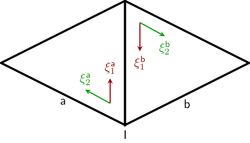
Consider two triangle cells and on a two-dimensional mesh, separated by interface as shown in figure 80. Each triangle cell has been assigned a barycentric parameterization with parent coordinates and . These cells have their parameterizations oriented such that the parameters on cell and the parameter on cell each point parallel the interface (although in opposite directions). Let parameterize the shared interface , and be defined as . The degree assigned to cell is , and the degree assigned to cell is . All barycentric index tuples on the two triangle cells are expressed with two indices and corresponding to barycentric coordinates and . The remaining index corresponding to is omitted, but is implicitly defined to be equal to (where is the degree assigned to the respective triangle cell).
Figure 80: Two triangular cells separated by interface on a two-dimensional mesh. We consider building the continuity constraint on the derivative of order on this interface.
A piecewise polynomial with support over and can be written in Bernstein form as
For an interface that is adjacent to a triangle, we are only required to consider the constraint on the derivative of order . We can write the continuity constraint on the derivative of order across the interface as and if we can enforce the above equality constraint by instead enforcing In the case that , we define . The degree-elevation operator is used here to map the respective Bernstein coefficients to a degree Bernstein space on the shared interface. Substituting in and rearranging yields the constraints in homogeneous form