20 Structural Elements
20.1 Summary
Beam and shell theories are important as they can greatly reduce simulation time when compared to solid formulations. Here, we develop a unified theory for solids, shells, beams, and rigid bodies showing that they are tightly related to each other. This includes showing that the same partial differential equations govern all four cases. This theory allows a wider application of beams and shells since we now have a consistent framework within which we can directly incorporate all nonlinear material models developed for standard solid formulations.
Of particular importance is that we do not arbitrarily eliminate higher-order strain terms in our unified theory [9, 119]. This vestigial practice was primarily motivated by the limitations of low-order FEA since the linear basis functions cannot approximate these higher-order strain terms anyway. However, by retaining those higher-order strain terms our theory remains consistent and, by leveraging higher-order, smooth splines to approximate them, we can achieve greater accuracy and robustness in computed solutions to structural theories. Also, while not treated here, we anticipate this clean and concise theory to aid us in our search for locking-free beam and shell numerical approximations to the continuous theory.
Additionally, we make an initial attempt at implementing an FRM shell. As part of this, we show that drilling stiffness can be implemented as a slight modification the stress state.
20.2 Previous work
This work assumes a basic understanding of continuum mechanics and associated concepts. For a basic overview of continuum mechanics there are many resources, but [75] is a great starting place.
Within the realm of IGA, beam and shell theories are dominated by theories where the higher-order terms of the Green-Lagrange strain are thrown away so that it becomes linear in the strains defined on the mid-geometry. A somewhat recent example of this for beams can be found in [9], while an example for shells can be found in [119].
However, there are beam and shell theories that do not discard the higher-order terms. This is done by working with the deformation gradient instead of the Green-Lagrange strain. This has the added benefit that a wider range of material models can be used. The origin of such theories can be found in Reissner beam theory [77, 78, 79]. Rather than degenerating a classic three-dimensional continuum model, Reissner assumed a form for the strains and that the resultant forces and moments were some function of those strains. This theory was extended by others such as in [48, 92, 98]. The issue with this theory is that the material law is not tied back to three-dimensional continuum mechanics and can be rather hard to decipher. A solution to this issue was proposed in [7] where it was shown how to decompose the deformation gradient into the assumed strains of Reissner beam theory. However, this was only for straight beams. An attempt to extend this to curved beams was made in [61], though this was incorrectly done as the curvature of the beam was not properly handled. A deeper explanation is given in Deformation gradient and local bases.
For shells, a very similar theory can be found in [17, 70, 72] which finds its foundations in the series of papers [93, 94, 95, 96, 97]. This theory is interesting because the strain measures proposed there can be recognized as generalizations of those from Reissner beam theory though that connection is not recognized there. This connection is made even more obvious in later papers [24, 71] where beams and shells are both treated with the same equations as those in Reissner beam theory. The authors were able to also show the connection to the deformation gradient. One issue with this theory is that the authors primarily dealt with triangular elements which has little applicability to IGA.
20.3 Geometric description
The most general structural element in Finite Element Analysis (FEA) is the traditional solid element. It can be used to simulate how any three-dimensional solid body will deform and displace. However, for efficiency, assumptions about the deformation of the solid body are made so as to simplify the physics of the body. Examples of this are shells, beams, and rigid bodies. In each of these cases, the physics are reduced to a lower dimensional manifold; for shells to a two-dimensional manifold, for beams to a one-dimensional manifold, and for rigid bodies to a zero-dimensional manifold. This manifold is known as the mid-geometry while the dimensions left over from the dimensional reduction to the mid-geometry are known as the section. A more precise definition of the section will be given later.
This leads to a set of four structural elements indexed by , which is the dimension of the manifold to which the physics are reduced. In the following, we will call this an -dimensional structural element. The index must obey the following inequality.
Note that when , there is no dimensional reduction and the structural element is just a solid element.
Since these theories are defined with indices, we can then use indicial notation to represent all of these elements using the same partial differential equations. This includes using the Einstein summation convention. This is done by specifying three different sets of indices.
The superscripts and are used because, as we will see, those indices are typically used to denote quantities in the mid-geometry and section, respectively.
In order to simplify notation, we use different types of indices to indicate which set the index comes from. A Latin index indicates that it comes from , i.e., , and a Greek index indicates , i.e., . Since is the complement of in , we use primed Greek indices to indicate , i.e, .
We note that we only consider manifold mid-geometries. There are many methods handling non-manifold mid-geometries, however we do not treat any of them here.
20.3.1 Reference configuration
In order to better understand the quantities in this and the following sections, the reader is referred to figure 144 where a beam example is presented.
In an -dimensional structural element, the physics are reduced to a smooth -dimensional manifold known as the mid-geometry and denoted by in the reference configuration. We can locally parameterize this manifold meaning that each point in a neighborhood in can be uniquely mapped to a point in . Letting be that point, we can then let locally represent a smooth invertible function, i.e., .
Attached at every point is a subset of a -dimensional affine space known as a section. Choosing a point , the corresponding section is then denoted by . Recall that the mid-geometry is parameterized locally by , meaning that a section can alternatively be denoted by . In fact, this can be done for any mapping from .
As a section is affine, there exists a basis for each section, known as the directors, that spans it. The directors consist of linearly independent vectors in and are denoted by in the reference configuration. Letting , then there exists a unique vector such that Since the directors must be linearly independent, can be uniquely represented by providing a nice parameterization of the section.
This demonstrates the affine structure of a section. The point in the section is created by translating by a vector , which is from an -dimensional linear space. Finally, since the directors are attached to a section, they can also be parameterized by , i.e., .
Letting denote the reference configuration of the entire body, it can then be defined as Additionally, requiring that the sections not intersect means that there exists, for each point , a unique pair of vectors such that , , and . The parameterizations of the mid-geometry and the sections can then be pulled through, allowing to then be locally parameterized by . Let , then
Letting be the boundary of and be the boundary of , we can construct the boundary of by partitioning it into the following two sets.
We then assume that the boundary of , denoted by , consists solely of these two sets. This assumption is violated when the section do not continuously change over . An example of this occurs when the thickness of a shell suddenly changes from one value to another. In such cases, there is an inconsistency in the stress state between neighboring sections due to the sudden change in the section. However, in practice this assumption is often ignored.
An important distinction in the previous definition is that and are boundaries in their corresponding subspace topologies and not the topology of . To see the distinction consider the boundary of the mid-geometry, , of a rigid body. In this case, the mid-geometry is just a single point, resulting in the boundary being that single point again in the topology of . However, in the subspace topology, the boundary would instead be the empty set, .
20.3.2 Current configuration
The current configuration at time , denoted by , is found through the deformation map, , which is required to be smooth and invertible. A wide class of elements in use currently also require the assumption that sections must map affinely into the current configuration. This assumption means that each section, when treated in isolation, will only translate and deform by a linear operator. This generates a field of translations and a field of linear operators both over .
Recall is itself an affine structure, which means that is also an affine structure. Letting , there exists a unique vector such that where Due to the structure of , we can define a deformation mapping of the mid-geometry from the reference into the current configuration; .
which in turn defines the mid-geometry in the current configuration as Consider the case of a hollow tube. The mid-geometry passes through the middle of the hollow space inside the tube without ever touching the tube itself. Thus it is not necessarily true that . For simplicity, in such cases we assume to be smooth and invertible just like .
Mapping the directors into the current configuration and recalling that is uniquely represented by in this basis, we can alternatively say that through the linearity of . This demonstrates the affine structure of . The point in the section is created by translating by a vector , which is from a -dimensional linear space. Due to this, we let be the section in the current configuration and denote it by , where .
Figure 144: The relationship between the different quantities in the reference and current configurations for a beam.
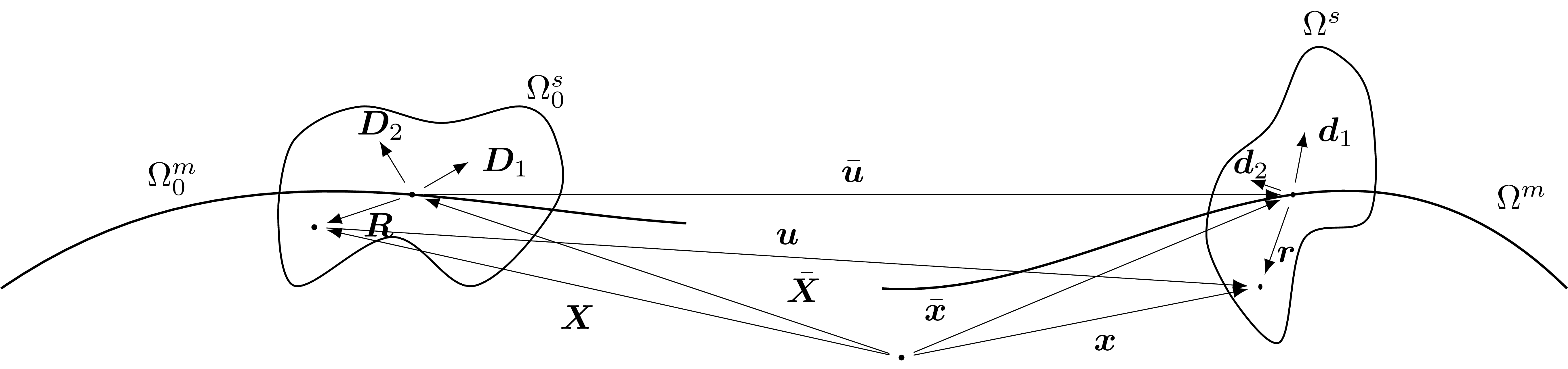
The result of all of this is that the current configuration is then Since is smooth and invertible, we can pull the parameterization of through to . Let , then Additionally, the displacement map is given by the traditional expression
Using the deformation maps, we can also map the different boundary sets from the reference into the current configuration;
A wide range of structural elements fall into this paradigm, including continuum based elements like those found in [12]. We, however, will additionally assume that sections can only move rigidly. This means that the set of allowed linear operators is limited to , i.e. rotation matrices. In other words
It might not be immediately obvious how solid elements fit into this paradigm as typically they are not described as having sections. This is because the orientation of the section can be ignored as they are zero-dimensional, i.e. a single point. Thus the rotation field can be arbitrary.
20.3.3 Deformation gradient and local bases
The deformation gradient is the gradient of the deformation mapping , though it is often shorthanded to This gradient is important because it allows us to translate derivative quantities between the reference and current configurations. The determinant of the deformation gradient, , is also important as it transforms volumetric integrals between the reference and current configurations.
Closely related to the deformation gradient are the covariant and contravariant bases, though first, we need to define some derivative notation. Let be an arbitrary function parameterized by and time , then a derivative of with respect to is denoted by We also use dot notation to denote the total time derivative of a quantity.
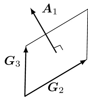
In table 16 we provide the definition of the contravariant and covariant bases. Note that the representation of some of the quantities is notationally simpler, but there are representations that are computationally simpler. As part of defining the covariant basis, we also define the directional area vector and the integral pullback. The directional area vectors are just the vectors normal to the parallograms whose sides are given by two of the contravariant basis vectors. See figure 145 for an example. The length of one of these vectors is just the area of the corresponding parallogram. The integral pullback will pullback volumetric integrals in the reference or current configuration to the parameteric coordinates . Note that denotes the Levi-Civita symbol. It is easy to verify the defining relationship between the contravariant and covariant bases, i.e. where denotes the Kronecker delta.
Reference Configuration
Current Configuration
Relationship
Contravariant Basis
Directional Area Vector
Integral Pullback
no sum over
no sum overCovariant Basis
Table 16: Contravariant and covariant bases with related quantities. Includes both the reference and current configurations as well as the relationships between.
Figure 145: The directional area vector which corresponds to the parallelogram defined by and
The deformation gradient and its inverse in terms of the contravariant and covariant bases are then
where denotes the outer product or tensor product of two vectors. By recognizing that we can define strain measures and decompose the deformation gradient into them. The map constructs a skew symmetric matrix from an axial vector while extracts the axial vector of a skew symmetric matrix. consists of the membrane and shear strains while are the curvature strains. These can be recognized as the strain measures of Reissner beam theory [77, 78, 79]. The decomposition of the deformation gradient is then which is a generalization of the decomposition in [7]. We note that specializing this for beams and the assumptions of [61], we do not recover the deformation gradient presented there even though it was supposed to be a generalization of [7] also. They are missing the contibutions of the determinant of the Jacobian of the reference geometric map, specifically the contributions of that determinant to the covariant basis. At the centroid, under their assumptions, the determinant is one, recovering their expression. However, the determinant varies over the section due to the curvature of the beam causing our definition for the deformation gradient to differ from theirs away from the centroid.
Finally, gradients in the different configurations can be found using the covariant bases. Let be an arbitrary function parameterized by , then the gradient in the reference configuration and the current configuration are, respectively,
20.4 Partial differential equations
Before considering the partial differential equations, we need to consider the domains that boundary conditions will be applied to. The different boundary conditions for the PDEs are applied to different portions of the boundary. We do this by subdividing the boundary of the mid-geometry, , and then constructing subdivisions of . If is subdivided into and such that then we can define the subdivisions of as It is fairly simple to show that This subdivision is necessary because of the rigid body motion assumption. The displacement is really only defined on the mid-geometry and so the boundary needs to be subdivided based on the mid-geometry. We cannot arbitrarily subdivide the entire boundary.
The strong form of the governing equations are Note that the Neumann boundary condition over is zero. Non-zero Neumann boundary conditions over are typically handled by lumping them in with the external body forcing once it has been reduced to the mid-geometry. For simplicity here, we eliminate this manipulation.
The strong form over can be converted to a strong form over by converting to and from a weak form. This requires a space of test functions, which incorporates the rigid-body motion assumption. First, the variation of is found.
Letting be the axial vector of the skew symmetric matrix Thus the test functions are These test functions represent every possible variation that corresponds to the kinematic assumptions.
The weak form of solid continuum mechanics is then We focus on the conversion of the two most complicated equations, i.e., the conservation laws. The boundary conditions are much simpler and can also be converted using similar techniques to what follows.
We combine the two conservation laws into one by adding together equation and equation and applying the divergence theorem to the stress term in equation . This makes sense because the test functions are arbitrary as long as they follow the kinematic assumptions, allowing us to eventually separate out two new conservation laws tailored to the n-dimensional structural element. Recognizing that is just the identity operator, we can make the following simplification This is the first step that reduces the physics to the mid-geometry. Note that since , , and are parameterized by , the weak form can be simplified to the following form. Also, the area integral is reduced to due to the traction being zero over .
The stress term on the right is now only summed over the indices having to do with the mid-geometry.
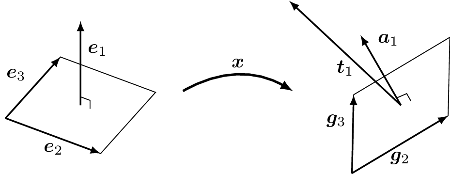
Using , we pull back the volume integrals to the parametric coordinates. We can also do so for the area integrals using a variation of Nanson’s formula. where is the classic Cartesian basis of . The quantity is simplified by recognizing over and the left over components, , are just the parametric coordinates of the normal vector of boundary of the mid-geometry. Substituting all of this back in We define the internal tractions as
These internal tractions are physically significant. Consider a differential area in parametric coordinates whose normal is . The internal traction is just the traction over this area when it is mapped into the current configuration, as seen in figure 146.
Figure 146: The mapping of a directed area, , from parametric coordinates to , a directed area in the current configuration. The traction over this area is then just .
Using Fubini’s theorem, we break apart the integrals into integrals over the section and the mid-geometry. Letting be a differential portion of the mid-geometry, a differential portion of the boundary of the mid-geometry, and a differential portion of the section we can say This is possible because of the pull back to the parametric coordinates where parameterizes the mid-geometry and the section. Along with replacing the left over test functions with their definition, we now substitute these integral splits.
Evaluating integrals over the sections, reveals the resultants. Note that we have also provided the resultants for the Neumann boundary condition in equation . In order to do so, we pulled the area integrals back to the parametric coordinates with .
Substituting in all of the resultants, the weak form is then
The divergence theorem then says Recalling that and are arbitrary, we convert this back to a strong form.
20.5 Rotations
A rotation can be represented using the Euler axis-angle representation. Essentially, the direction of a vector can be used to represent the axis of rotation while the magnitude of that vector represents the angle of rotation around that vector. A rotation matrix can then be created using the exponential map.
This can be simplified to the Rodrigues rotation formula where . There is a small issue with this formula when the rotation is zero as it involves a divide by zero. However, this can be avoided many ways. One common way is to use small angle approximations of the sine and cosine functions. Another option is to use the sinc function, which should hide those considerations.
When considering dynamical simulations, it is common to use angular accelerations and velocities. Consider an arbitrary vector that is rotated to the vector The angular velocity is the vector such that and the angular acceleration is just the time derivative of the angular velocity.
The acceleration of is then
In FEA, it is fairly common to use the incremental rotation as it simplifies solving for rotations. At time , we can consider the rotation . The rotation rotation at time can then represented with where is the incremental rotation matrix whose Euler axis-angle representation is , which is a function of time. must be zero at .
We can greatly simplify things by recognizing that at This means that when we employ a time integration scheme and we solve for the acceleration, we are basically just solving for the angular acceleration at each time step. This also means that the discretization of the incremental rotation vector can be transfered to the angular acceleration and velocity. This means that the full angular acceleration and velocity can be stored as a field instead of at quadrature points.
Employing the central difference method, we can write the next rotation as The central difference method is often described as an explicit method. However, this is only ever true given the assumption that the problem is rate-independent. This assumption is often broken in the presence of damping and certain material models. Rotations also introduce a rate dependence. This is often handled by just replacing the velocity at time with the velocity at instead in the balance law used to solve for the acceleration. This is an approximation, but it is just one on a long list of approximations we make in order to make explicit dynamics fast.
20.6 Weak form
Recognizing that the variations of the strains are and setting the variations and to zero on , the weak form, equation , becomes where
20.6.1 Variation of the internal force
Recall that the internal residual is given by The rotated internal forces and moments can be simplified to the following form so that the only changing quantity is the rotated traction over the section. After a pull back of the Cauchy stress to the second Piola-Kirchhoff stress, the rotated tration is The variation of the second Piola-Kirchhoff stress is given by where is the moduli matrix in the reference configuration and the variation of the Green-Lagrange strain is given by The symmetries of then imply Recognizing that and , the variation of the rotated traction is then The resultant moduli matrix is then where Thus Note that if a material model is associative, then the resultant moduli matrix is symmetric.
Taking the second variation of the strains the variation of the internal residual is then
20.7 Material models
Using material models typically used for solid elements directly in shell and beam elements will result in an overly stiff response. This is because the assumption that sections remain rigid typically results in a stress state that is inconsistent with equation . This is typically handled by modifying the strain state such that certain components of the stress are zero.
Crucial to this is the so-called lamina basis [45]. At every point a set of basis vectors, represented by , is defined so that they align with the laminae of the geometry. Normal to these vectors is a -dimensional space and we let represent a basis for this space. This basis can be arbitrary as long as
The theory is simpler with an orthonormal basis, equation , because it avoids having to deal with the metric tensor in the reference configuration. Collectively, these two sets of basis vectors form a basis for and are known as the lamina basis. An example of this basis can be seen in figure 147.
Figure 147: The laminae through the thickness of a shell with the lamina basis for one of those laminae.
We want to set any component of stress that is normal to the laminae to zero. In order for this constraint to make sense in both the reference and the current configuration, must transform contravariantly while transforms covariantly. Thus a push forward of the second Piola-Kirchhoff stress to the Cauchy stress implies Equation provides the push forward of tangent space of the laminae, while equation ensures that will always be normal to that tangent space.
We can find the additional deformation, denoted by , with two assumptions. The first assumption is that all additional deformation must be normal to the laminae. As the stress must be zero in that space, we adjust those components of deformation. Mathematically, this means where denotes the right Cauchy-Green tensor. The second equation can readily be recognized as the constraint used in traditional structural theories. This assumption implies that the additional deformation takes the form where is the basis dual to defined by where However, equation does not constrain all of the components when . This is solved by the second assumption, which is that is the least amount of additional deformation that satisfies equation . Mathematically, The solution to this minimization problem is . The unknowns and constraints are now balanced, allowing us to solve for the unknowns with a Newton-Raphson loop.
The rest of this section is devoted to proving that the second assumption implies . Equivalently, this assumption is given by
In order to solve the minimization problem, we require the inverse of the matrix and denote this inverse with . exists if and only if is invertible. First we prove that if is invertible then is also invertible. This is done with a proof by contradiction. Assume that is singular. Thus there exists a non-zero vector in denoted by such that . Now consider the following decomposition of the modified deformation gradient Applying the modified deformation gradient to Thus we have found a non-zero vector in the null space of . Therefore is singular as well. Thus if is invertible, then is also invertible and exists.
Now we prove that if is invertible, then is also invertible. Using a variant of the Woodbury matrix identity, we find This inverse can be readily confirmed through multiplying with this candidate inverse. Thus, by combining this result with the previous result, we can say that is invertible if and only if is also invertible.
Now that we have shown that exists for all valid configurations, we can solve for the least amount of additional deformation. If is the least amount of additional deformation, then its components are symmetric, i.e., . To prove this, let us consider variations of the second Piola-Kirchhoff stress about a solution to the minimization problem, specifically the variations of the deformation gradient that produce no change in the stress state. Assuming that the map from the Green-Lagrange strain to the second Piola-Kirchhoff stress is locally smooth and invertible, we only need to consider variations of the Green-Lagrange strain about a solution. This smoothness assumption is standard for most traditional elements. Consider the Green-Lagrange strain constructed from .
Consider the directional derivative of in the direction Thus moving in the direction will not affect whether the solution satisfies the stress condition equation . Thus we can take the directional derivative of equation in that direction and set it equal to zero without worrying about how the stress condition affects it.
Thus by running through its possible values. Recalling the definition of proves .
20.8 An FRM shell
As part of an initial exploration of applying FRM to shells, we now specialize the theory for a static Reissner-Mindlin shell.
Reissner-Mindlin shells suffer from drilling singularities due to depending on the rotation through the single director . Thus, the rotation is not fully defined. Any additional rotation about the director would leave the director unchanged.
This is handled by adding artificial stiffness. One method is to use the polar decomposition to find a rotation [36]. A rarely mentioned defining feature of the polar decomposition is that the resulting matrix is the closest rotation matrix to the deformation gradient under the Euclidean norm [15]. Combining this with the constraint that the reference directors have to rotate to the current directors, the rotation matrix can now be uniquely defined by Note that when the classic polar decomposition is recovered. Solving this minimization problem at the midsurface of a shell leads to the constraint where This is a slight generalization of constraint in [36].
We can enforce this constraint with the penalty method, for which the cost function is where is the drilling stiffness. As the only dependence on the current configuration is through the strain, we can define a drilling internal force and combine it with the internal force in equation and equation . Similarly, a drilling moduli matrix can be defined and combined with the moduli matrix in equation . Thus drilling stiffness can be handled with a simple modification to the material model.
20.8.1 The matrix form
Even though we only implemented a linear theory, we present the nonlinear matrix form here The linear form is practically identical.
Discretizing the problem, the nodal matrix form of the residual is where After assembly, the equation we solve are This equation can be solved with a Newton-Raphson loop for which the nodal matrix form of the stiffness matrix is where Note that is not symmetric. In practice, it is often symmetricized such as in [30].
20.8.2 Body fitted verification
In order to have confidence in the shell implementation before running FRM simulations with it, we ran three of the standard shell benchmarks. All three are static body-fitted simulations.
The first benchmark is the pinched cylinder benchmark. The pinched cylinder consists of a full cylinder of length , radius , and thickness as shown in figure 148. Due to symmetry, only a quarter of the geometry is modelled. Two opposing forces of magnitude are applied to the middle of the shell. The elastic modulus is and Poisson’s ratio is . Several simulations with various mesh sizes and different spline degrees are performed. The vertical displacement at the application loading point is compared to the reference found in [29]. As shown in figure 148, refining the mesh or increasing the degree improves the accuracy of the result.
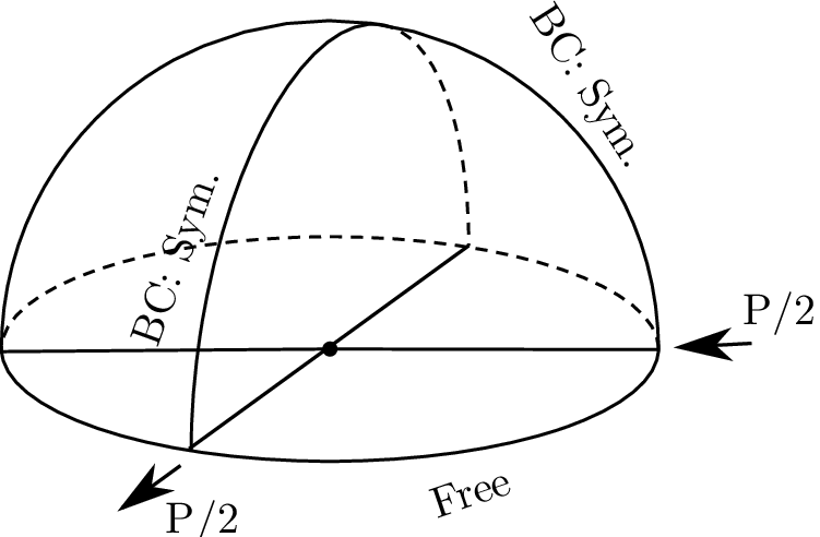
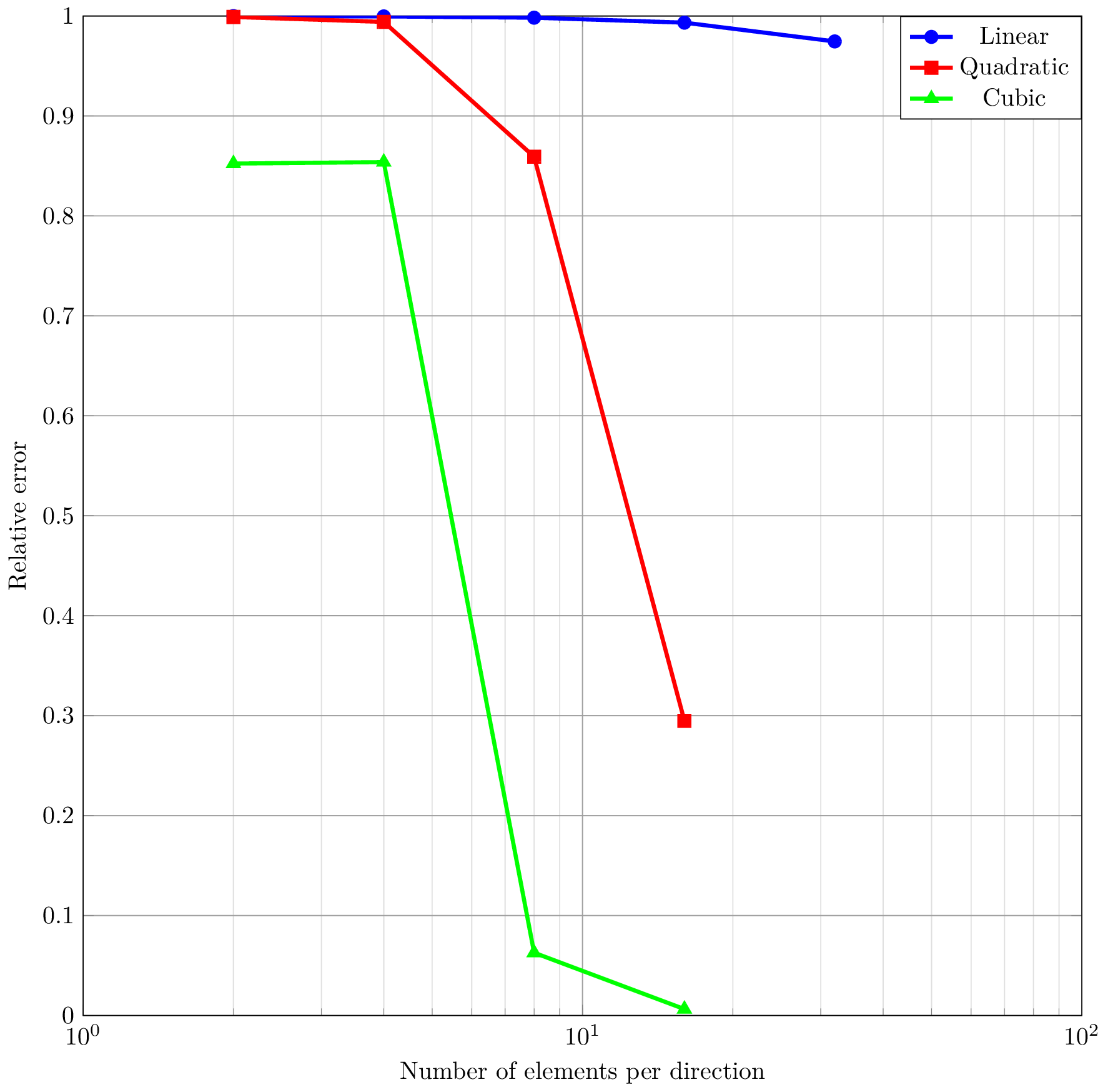
The second benchmark is the pinched hemisphere benchmark. The pinched hemisphere consists of a full hemisphere of radius of and shell thickness as shown in figure 149. Due to symmetry, only a quarter of the hemisphere is modeled. Two opposing forces of magnitude are applied to the shell. The elastic modulus is and Poisson’s ratio is . Several simulations with various mesh sizes and different spline degrees are performed. A reference solution for the radial displacement at the loading point can be found in [29] and is . As shown in figure 149, refining the mesh or increasing the degree improves the accuracy of the result.
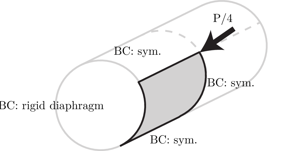
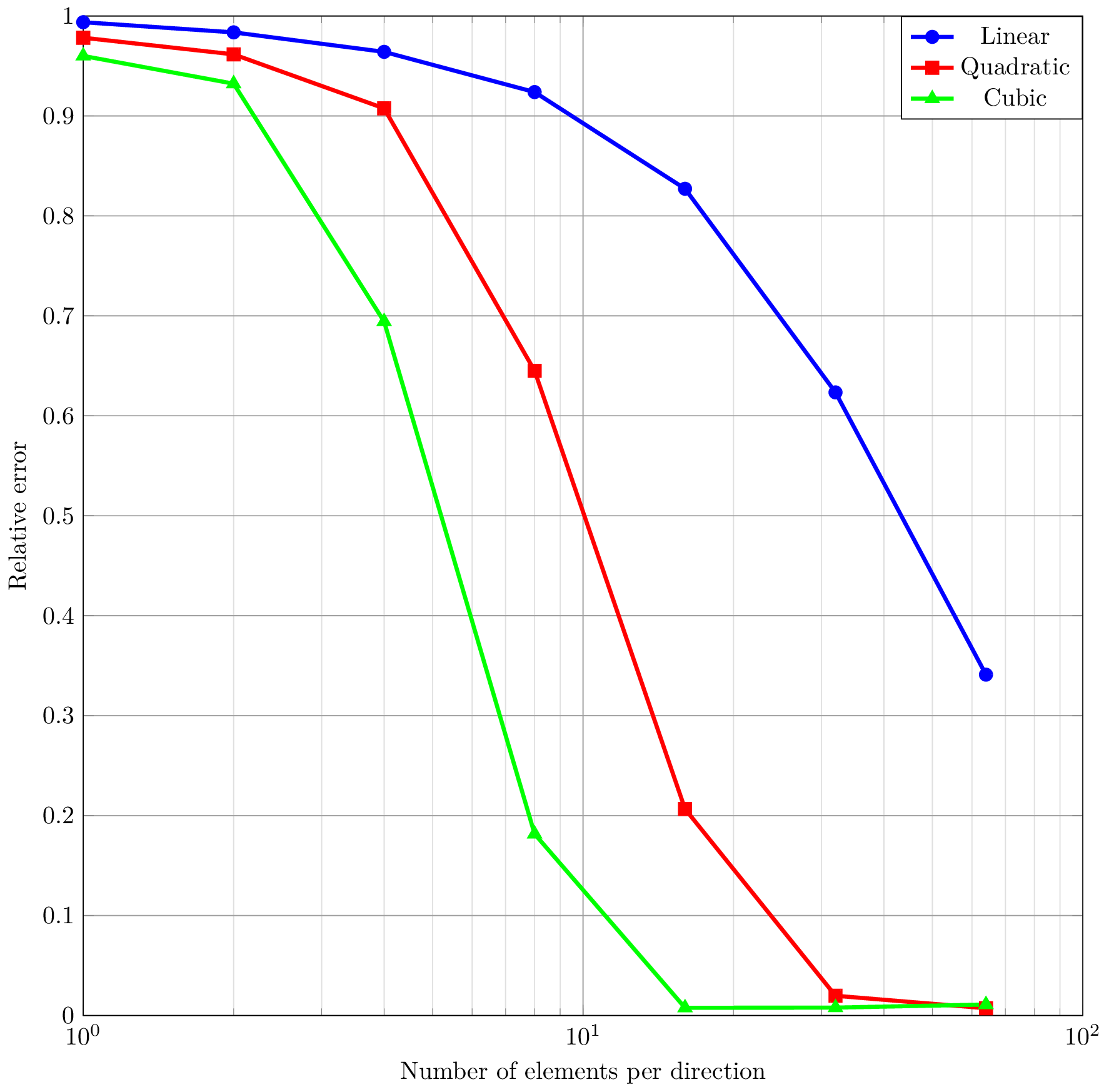
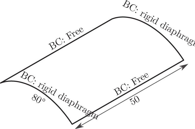
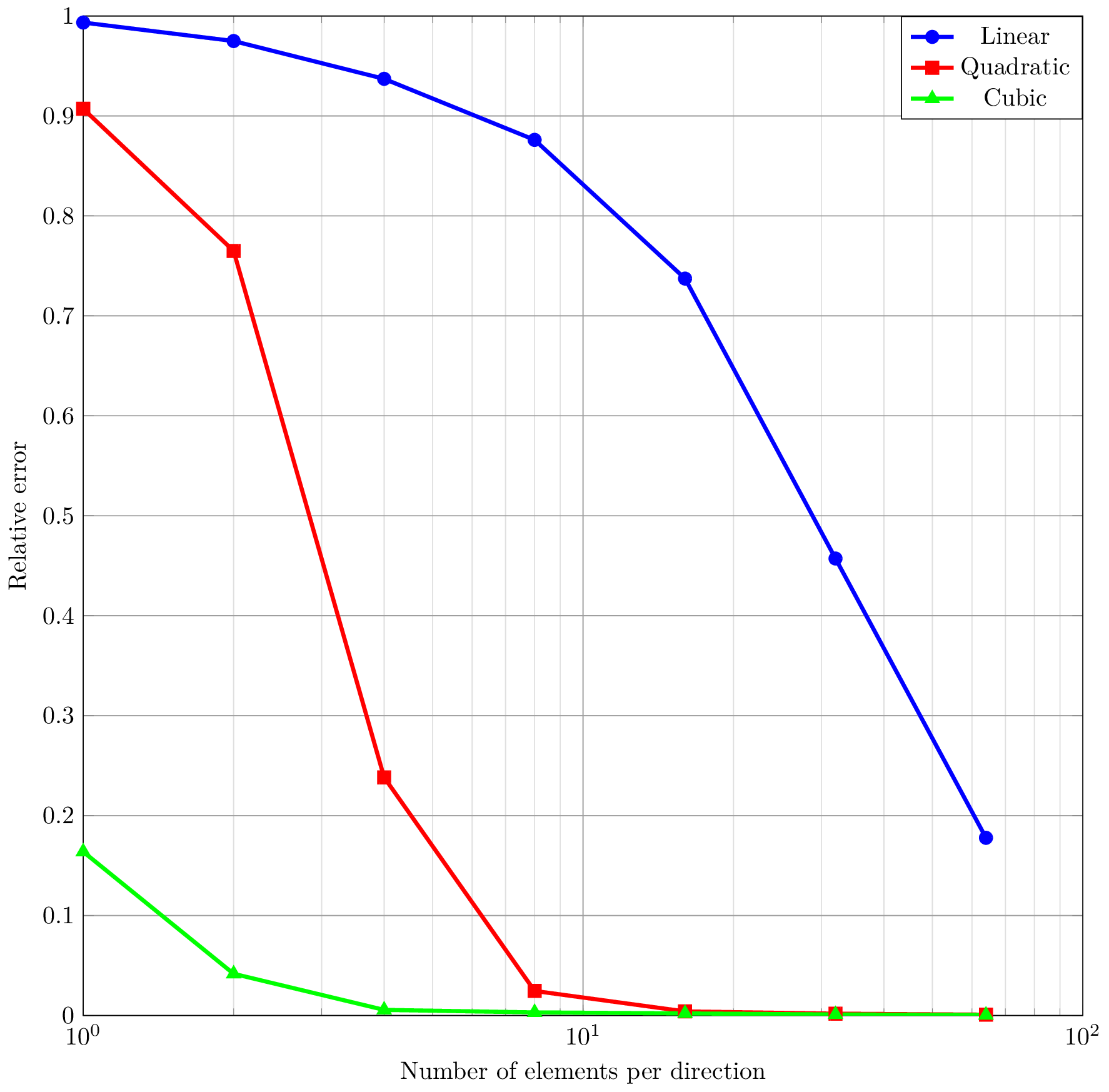
The final benchmark is the Scordelis-Lo roof benchmark. The Scordelis-Lo roof consists of a section of a cylindrical shell with length , section angle of , radius , and shell thickness of as shown in figure 150. The roof section is subjected to a distributed load of magnitude . The elastic modulus is and Poisson’s ratio is . Several simulations with various mesh sizes and different spline degrees are performed. A reference solution for the displacement along the lateral side at the midpoint can be found in [29] and is . As shown in figure 150, refining the mesh or increasing the degree improves the accuracy of the result.
20.8.3 Aspects of the FRM for shells
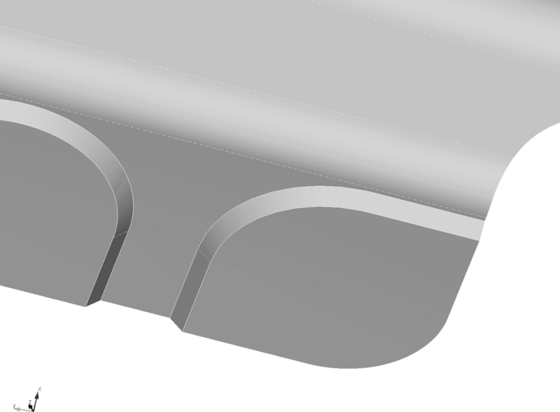
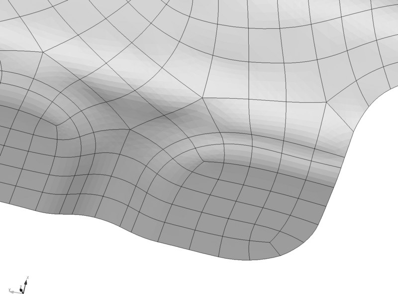
Shells are an excellent opportunity to exercise the FRM. However, building a simulation geometry that truly envelops the physical domain for shells is difficult due to the projection error generated from converting the CAD representation to a U-spline representation. For example, consider the three geometries in figure 151 wheere a CAD geometry is simpified into an envelope domain, from which a U-spline is created. This process leads to projection error as seen in figure 152, creating difficulties for FRM. We could greatly reduce this projection error by slightly changing the U-spline basis, however, we cannot completely remove it.
Figure 151: The three different representations of the second shell problem.
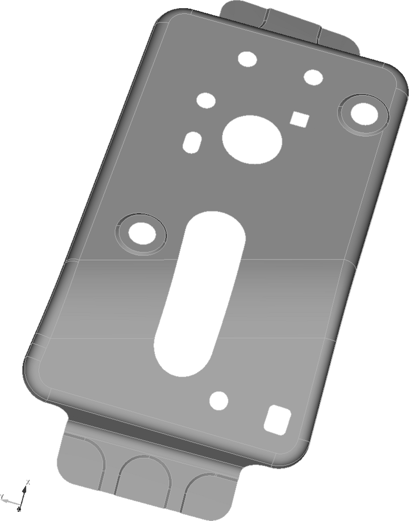
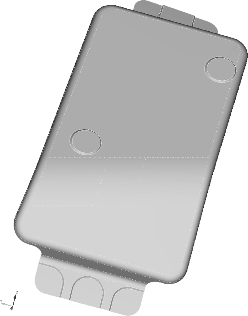
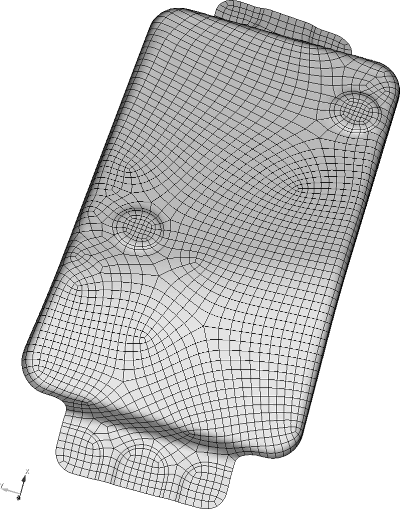
Figure 152: A close up of an envelope domain and the corresponding U-spline representation showing the projection error.
FRM requires a robust test of whether a point on the U-spline is inside or outside the physical domain, which is frustrated by the projection error. Notice that the projection error in figure 151c is completely separated from the creation of the envelope domain in figure 151b. By reversing this process, we can again separate the projection error from the actual inside outside test.
Returning to the definitions from (part "frm-envelope"), this algorithm is more concretely given in the following. Given a CAD manifold, denoted by , we can partition it into all of the different trimmed surfaces that make it up. This partition is denoted by and each surface is denoted by . An example of is shown in figure 151a. Additionally, we denote the CAD envelope with . An example of is shown in figure 151b. Similar to , we can partition into all of the different trimmed surfaces that make it up. This partition is denoted by and each surface is denoted by . Finally, the U-spline envelope domain is denoted by . A partition of is denoted and each cell is denoted . An example of is shown in figure 151c.
The algorithm for the inside outside test for shells is shown in algorithm 10. This uses several of algorithms developed in Bounding Volume Hierarchy. The input typically comes from . Note that the tolerance, denoted by , accounts for not being watertight and for deviations between and .
◾ Pseudocode for the inside outside test for shells
1: procedure shellInsideOutside()
2: ▷ Get an upper bound on distance to nearest point on
3: surfaces = ▷ Get the set of surfaces in nearest to using a BVH. Use to account for differences in and
4: if surfaces is empty then
5: return outside
6: end if
7: surfaces = ▷ Get the sorted set of surfaces in nearest to using a BVH
8: ▷ Initialize the distance to the upperbound on the distance
9: ▷ Leave the closest point on uninitialized
10: for each in surfaces do
11: if then
12: break loop▷ Truncate the search as there is no better solution in the rest of the surfaces
13: end if
14: = nearestPointOnSurface(, )▷ Search the surface for the nearest point. This is a CAD kernel operation
15: ▷ Compute the distance to the candidate point
16: if then▷ Check if the candidate solution is a better solution
17: ▷ Update the distance with the candidate distance
18: ▷ Update the solution point with the candidate point
19: end if
20: end for each
21: sort surfaces by and then
22: for each in surfaces do
23: if then
24: return outside▷ Truncate the search as there is no way for the point to be inside any of the other surfaces
25: end if
26: if distanceToSurface(, ) then▷ Check if the point is close enough to the surface. This is a CAD kernel operation
27: return inside
28: end if
29: end for each
30: return outside
31: end procedureAlgorithm 10: Pseudocode for the inside outside test for shells
As an implementation note, we used . We have access to the render facets from which we can construct as the set of the render facet vertices. This produces a much less conservative bound on the distance as the CAD surfaces can be fairly large relative to the U-spline element size.
A major simplification can be made by checking if entire U-spline cells are near the physical boundary or not. If they are far enough away, we only need to check one point to know if the entire cell is inside or outside. This check can be done with the BVH search in (part "sec:inverse-cells-near-cell") again using .
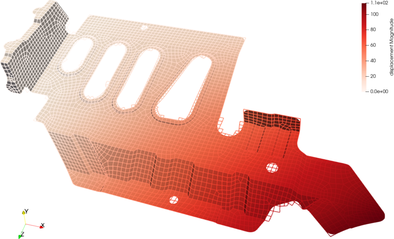
Applying the boundary conditions seen in figure 153 we run a simple simulation to verify that a valid quadrature rule can be robustly constructed. The results of the simulation are shown in figure 154. Even though there was significant projection error in certain locations, it was still able to construct a valid quadrature rule.
Figure 153: Boundary conditions for the second FRM shell example. The surfaces marked with Xs are clamped while the edges of the holes marked with arrows are pulled normal to the surface.
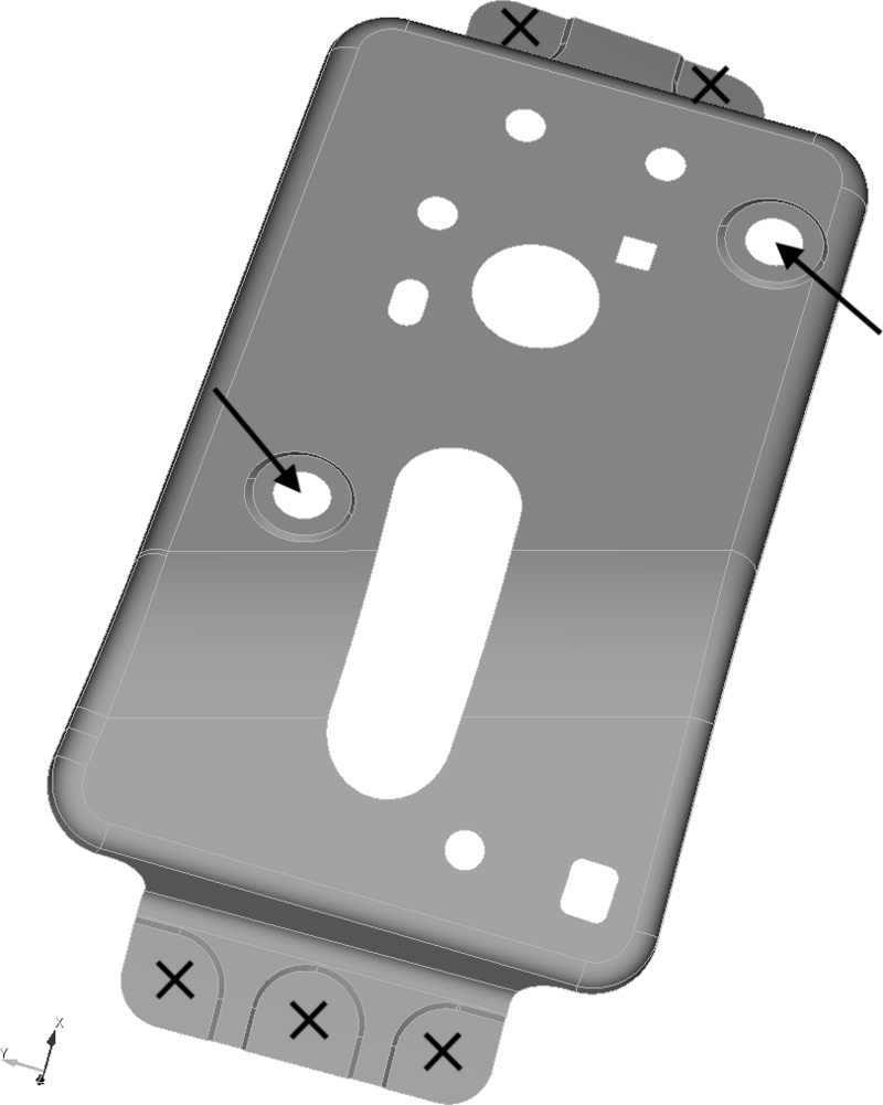
Figure 154: The simulation results for the second FRM shell example. The wireframe represents the envelope domain
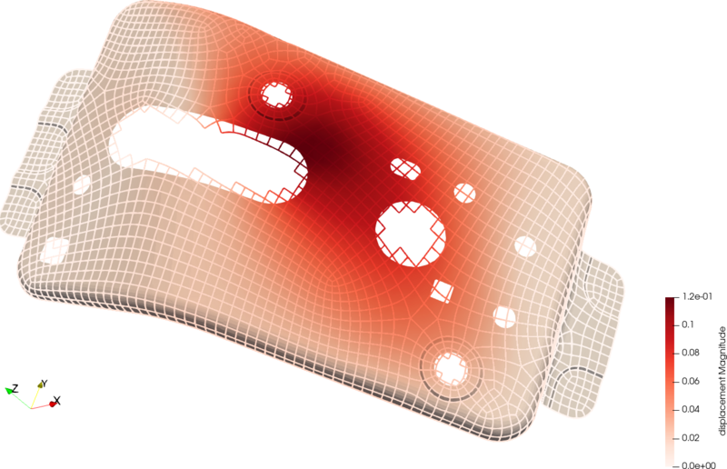
As a second example, consider the three geometries in figure 155 showing the construction of a U-spline for a simulation. It also suffers from significant projection error as seen in figure 156. Again, we could reduce the error by modifying the basis. However, this was not necessary in order to build a valid quadrature rule and run a simple simulation. The boundary conditions and results can be seen in figure 157 and figure 158, respectively.
Figure 155: The three different representations of the first shell problem.
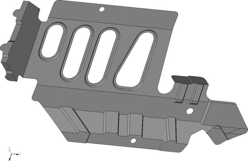
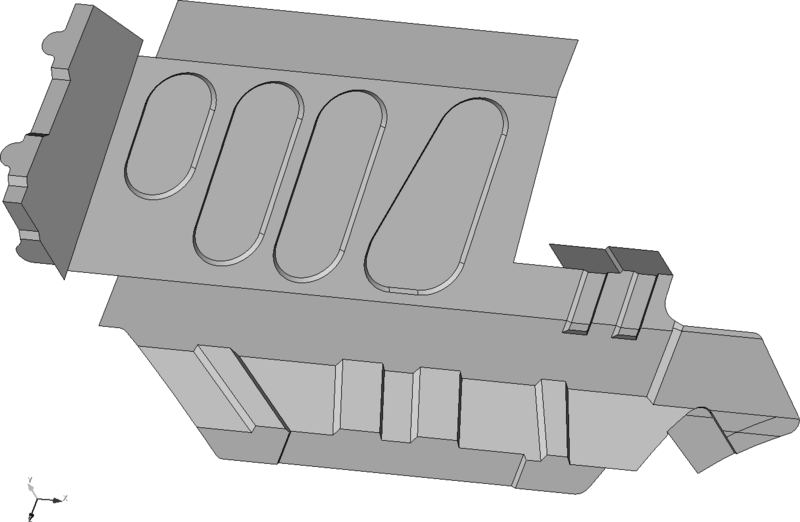
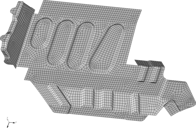
Figure 156: A close up of the envelope domain and the corresponding U-spline representation showing the projection error for the first example.
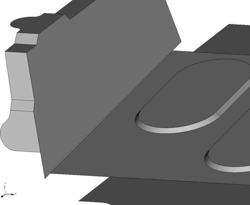
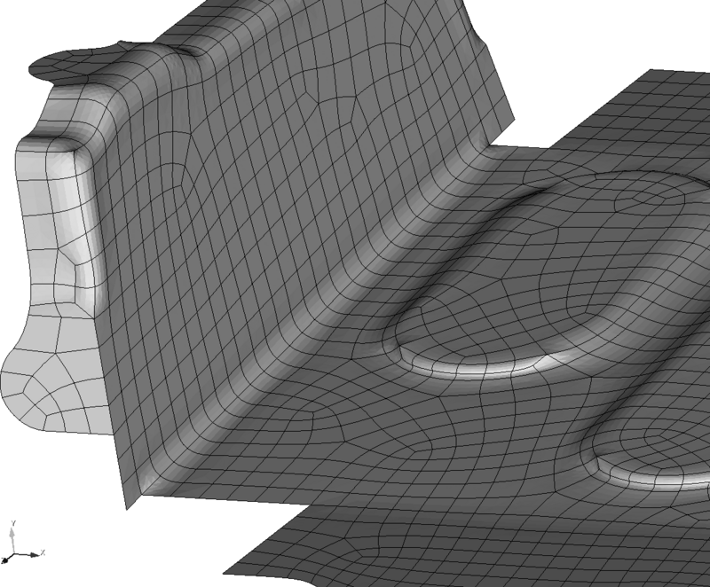
Figure 157: Boundary conditions for the first FRM shell example. The surface marked with an X is clamped while the edge of the hole marked with an arrow is pulled normal to the surface.
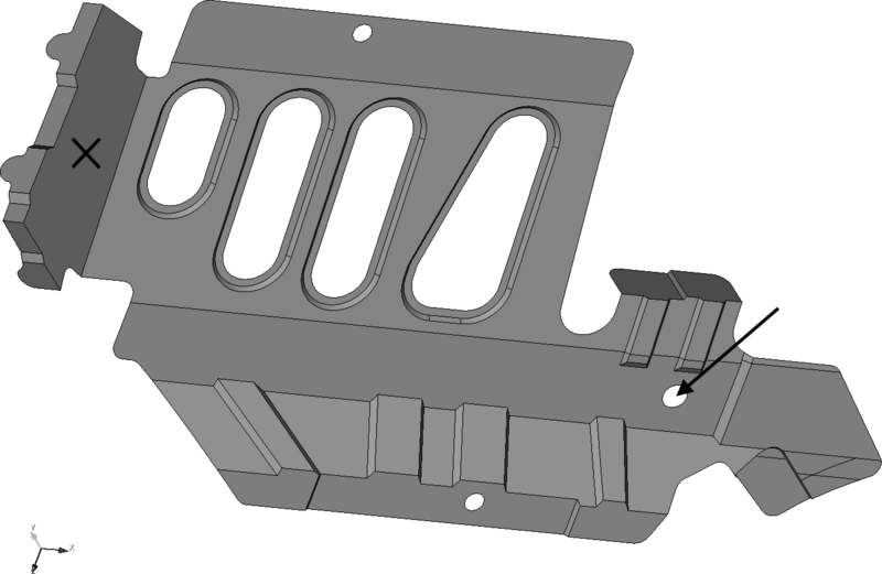
Figure 158: The simulation results for the first FRM shell example.