7 Inverse Mapping
7.1 An Overview of Inverse Mapping
U-spline fitting and trimming requires advanced inverse mapping algorithms to map points on the trimming surface to the parametric domain of the U-spline to be trimmed. To accomplish this, we solve a nonlinear optimization algorithm. Defining a distance cost function to minimize, the general inverse mapping problem is defined by the following minimization problem: where is the point we are inverting and is the U-spline manifold onto which we are inverting.
7.2 Bounding Volume Hierarchy
In practice, the manifold will be partitioned into segments or elements that can be used to accelerate the spatial search aspects of the algorithm. Bounding volume hierarchies (BVH) allow us to eliminate most of the elements as candidates for the element containing the closest point.
Given a partition of a manifold , a BVH tree is constructed using a bottom-up approach through the following steps:
Step 1: Each element in is first wrapped by a basic bounding volume.
Step 2: Every two bounding volumes are grouped into a larger bounding volume.
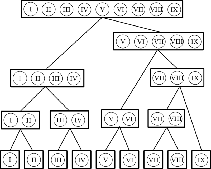
Step 3: Step 2 proceeds in a recursive manner, eventually resulting in a binary tree structure with a single bounding volume at the top.
Figure 90b: BVH tree built from segments in Figure 90a.
Figure 90: A BVH tree built from a partition of a U-spline manifold into nine Bézier segments. Note that the bounding volume type has not yet been specified.
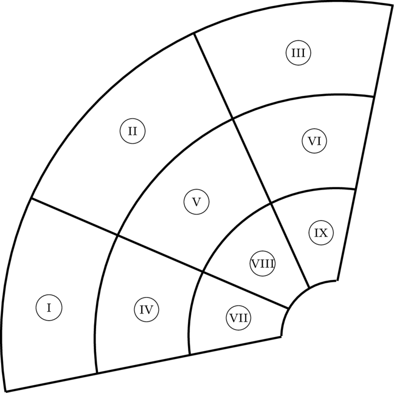
The choice of bounding volume type plays an important role in the efficiency of the search algorithm provided by the BVH tree structure. Generally, the bounding volume should have a simple shape so that less storage is required for the BVH tree structure and calculating upper and lower bounds on the distance between a point and an element is simple and fast. Additionally, the bounding volumes are expected to fit the elements tightly so that we search through fewer bounding volumes. Various bounding volume types are used for collision detection in the animation industry and for ray tracing in computational geometry, including spheres, axis aligned bounding boxes (AABB), oriented bounding boxes (OBB), -direction discrete oriented polytopes (KDOP), and convex hulls.
7.2.1 Nearest Cells Search
In point inversion, we find the set of points on a nearest to another set of points . The set could be a single point, a point cloud, the points of an element from the partition of a manifold, etc. Robustly accelerating point inversion requires an algorithm that can find a set of cells in that robustly contains the nearest points to . For simplicity, we only consider finding the cells nearest a bounding volume of . Note that a point is just a special case of a bounding volume.
Find all bounding volumes in the tree that overlap the given bounding volume
Find the nearest bounding volumes to the given bounding volume
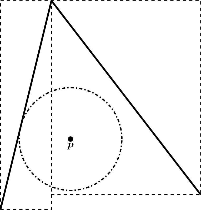
Figure 92: A simple example where the point lies outside of the bounding volume of the nearest cell, while lying within the bounding volume of another cell.
We could construct an algorithm that works by calling the second algorithm and then the first algorithm. However, this results in traversing the BVH twice.
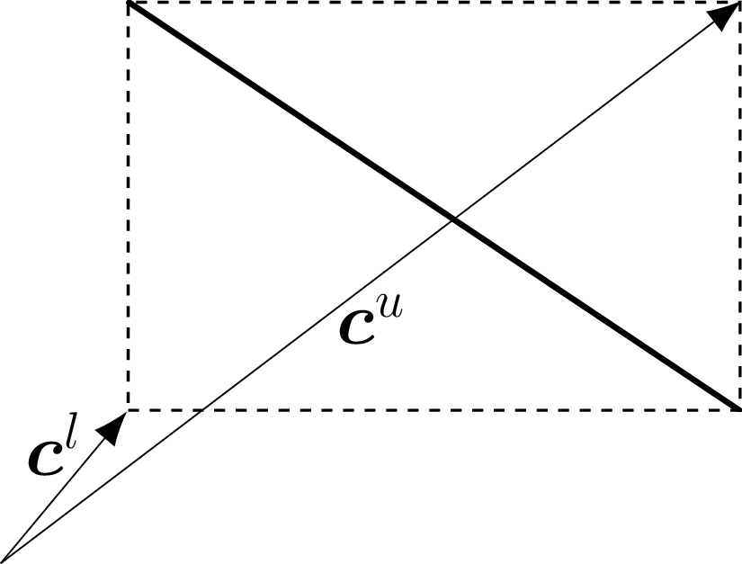
In the following we develop an algorithm that traverses the tree once and is guaranteed to find the correct set of cells. To facilitate this we define upper and lower bounds on the distance between points in two sets. Given the sets and , the strictest bounds are, by definition, However, from a practical stance, this strict upper bound does not lend itself to use in a BVH. As such, we define the lower and upper bounds, respectively, Note that the lower bound is equivalent to the strict lower bound while the new upper bound is looser. The benefit of these bounds is that they properly nest. Since and Thus, we can choose a convenient bounding volume for our query and then tighten the bounds as we traverse down each level of the BVH.
The set of cells nearest to is defined to be This set can easily be found using a BVH. Additionally, we might sort this set by the lower bounds as this can greatly speed up the search for the cell that is nearest .
7.2.1.1 AABB Bounds
AABB provide a simple method of computing the lower and upper bounds found at equation and equation . Given the sets and , these bounds simplify to where is the spatial dimension. The component in the sum in the lower bound is simply computing zero if the intervals of a single component of two AABBs intersect and the distance between the two intervals if they do not. This can be done using interval arithmetic and the so called clamping function.
7.3 Point Inversion
7.3.1 The General Approach
After finding the nearest cells using Nearest Cells Search, we can find the nearest point on a cell using In the following, the specific cell is often omitted from the inputs to the manifold except when clarity is required. Additionally, we restrict to be a tensor product of simplices. If we consider one-dimensional, two-dimensional, and three-dimensional cells, this class consists of lines, quadralaterals, hexahedrons, triangles, tetrahedrons, and wedges. Note that pyramids are the only common cell type that is excluded.
7.3.1.1 Point inversion over a simple simplex
For simplicity, we start by explaining the general approach of solving over a simplex rather than over a tensor product of simplices.
It is convenient to use barycentric coordinates to represent the parametric space when performing point inversion on a simplex. Recall that the barycentric coordinates of a unit simplex must satisfy the following conditions where is the dimension of the simplex. The equality constraint is known as the partition of unity constraint in the following. The convenience comes from recognizing that each of the inequality constraints represents one of the boundaries. A dimensional simplex has boundary cells, each of which is a simplex. Each boundary then has a parametric coordinate associated with it such that the parametric point is exterior if the parametric coordinate is negative, interior if it is positive, and on that boundary cell if it is zero.
The solution is then a stationary point of the following Lagrangian: where is the Lagrange multiplier of the partition of unity constraint, and and are the Lagrange multiplier and slack variable, respectively, of the th inequality constraint. The KKT conditions are then
This system has unknowns, however this number can be greatly reduced through an active constraint solution method. For active constraints, the number of unknown parametric coordinates are reduced to and occassionally an additional unknown Lagrange multipliers are needed.
The main step to enable this is a choice of basis for the parametric space or rather the tangent space to the affine space defined by the partition of unity constraint. This is because it eliminates the need to calculate . A basis for this tangent space must satisfy Additionally, we require any basis to satisfy the following requirements The first requirement allows us to reuse this basis for every dimension of simplex and after enforcing a new constraint. In the case of a new constraint, this is done by discarding the last vector and then permutting the rows of the left over basis vectors. Note that this requirement means that the last component of each basis vector is zero except for the last basis vector. Thus discarding the last vector allows us to move the zero at the end of each left over basis vector to the location of a new constraint while moving down all other values. For example, consider the basis for a triangle If the first parametric coordinate is then constrained, then we can construct a new basis by deleting . This leaves just which has a zero in the last position which can be moved to the position corresponding to the new constraint, moving all other values down. The resulting basis vector is
The second requirement on the basis vectors just maintains the expected behavior on a line domain. Line domains are simple to perform point inversion over without bringing in all the machinery needed by higher dimensional simplices.
The traditional basis of choice that satisfies all of these requirements is where represents the -th -dimensional Cartesian vector.
The main issue with this basis is that it is not orthogonal, resulting in a change in the residual norm when certain constraints are added or removed. In order to guarantee continuity of the residual norm, we instead choose another basis that is orthogonal in the parametric coordinate space: where is the -dimensional vector of ones and is the -dimensional vector of zeros. It is fairly simple to verify that each vector is orthogonal to and thus part of the tangent space. By entension, it is also simple to verify that each vector is orthogonal to each other due to the inclusion of and as subvectors. Note also that the norm of each vector is the correct length of .
Defining to be the permutted basis created by modifying the othogonal basis by the same procedure described above after enforcing new constraints, the residual reduces to A slight wrinkle is that we almost never actually have access to as the implicit coordinate is often condensed out automatically. However, we do have access to . Because these different bases span the same spaces, we simply have to find the transformation between the two. Given an arbitrary vector in the parametric space, The transformation between and is then where In the following, if a lowercase latin index is used to denote a derivative, it is defined to mean the following Given that this conversion is a linear operator, this definition simply extends to higher order derivative without considering the product rule. The residual then converts to which is now in terms of quantities that we have access to.
Defining another basis over the parametric space, , we can extract the Lagrange multipliers of the active constraints. Defining to be the set of active indices and to be the set of inactive indices, i.e. the active constraints, this basis is then where , is the first index in , and all other components are zero. Note there will always be at least one active index due to the partition of unity constraint. Thus is always well defined. The Lagrange multipliers are then Again, we represented the basis in terms of in order to represent the Lagrange multiplier in terms of quantities we have access to.
We can solve this system using a Newton-Raphson loop, for which the tangent is This tangent is not necessarily positive definite, meaning that the resulting search direction might not be a descent direction. If this is the case, we fall back to the gradient descent method.
Once a step direction has been identified, it must be converted back into the other basis representations. Denoting the step in terms of the basis by , in the barycentric coordinates it is However, just like how we only have access to certain components of the full gradient, we need to represent the step in terms of the basis. Denoting the step in that basis as , it is given by
7.3.1.2 Point inversion over a tensor product of simplices
The work in the previous section is generalized to tensor products of simplices by assuming that the parametric space of each tensor component is orthogonal to all other components. This essentially amounts to padding the basis vectors derived in the previous section with zeros before and/or after. Everything follows from that simple modification of the basis.
For example consider the case of a wedge element where the triangle domain comes first. The orthogonal basis is
The only wrinkle is when adding constraints, we need to discard the last basis vector from the correct set of basis vectors and then move the resulting zero from that set. Adding a constraint to the first parameter, the basis becomes This can be recognized as the basis for a quadrilateral element as we are now restricted to one of quadrilateral boundaries of a wedge element.
7.3.2 Optimizations
In the previous sections, we greatly sped up the algorithm by sorting the cells from the BVH as we can truncate the search once they were too far away from the point. In this section we make three additional optimizations to this algorithm. The first occurs when the gradient of the mapping is full rank, the second occurs when the mapping is an affine mapping, and the last occurs when a mapping is comprised of a mixture affine and nonlinear regions. We call a mapping comprised of a mixture of regions a composite mapping.
7.3.2.1 Full Rank Mapping
Given that is assumed to be a smooth injective map that maps into a -dimensional space, if is a -dimensional manifold and there are no active constraints, then then is a square invertible matrix. The residual can then be simplified down to resulting from being invertible. The tangent in this case is which always results in a descent direction as seen in the following: It is zero if and only if . If a constraint activates, we switch over to the previous method, but if all the constraints deactivate we switch back to this method.
The efficiency gains come in two forms. First, if this method is active at convergence, we know there is no better solution as is assumed to be injective. In this case, we can truncate the search without searching the rest of the cells even if their lower bound is zero. Second, we avoid many evaluations such as second order derivatives or checking that the search direction is actually a descent direction.
7.3.2.2 Affine Mapping
An affine mapping is defined by a translation vector and a linear operator. Given an origin point , an affine map can be defined with where is constant everywhere. The residual is where is the tangent, which is constant over the entire geometry.
The optimization comes in two forms. First, each cell only differs by a translation, allowing us to check all of the cells as one large block. Second, it eliminates the Newton-Raphson iterations in the general theory above as the tangent is just a constant operator. However, the correct set of constraints is still unknown. By generalizing the nonlinear approach in The General Approach to take an entire affine region instead of just a single cell, we can solve for the correct set of constraints. All of the basis conversion for adding and removing constraints is still valid. Every step in the algorithm will step to the best point under the current set of constraints and then either terminate or update the constraints.
A further optimization occurs when the affine mapping is orthogonal. This only possible when a the domain of the affine mapping is a tensor product of more than one components. If that is true, then the mapping is orthogonal only when whenever comes from a different tensor product component than . This decouples all of the components of the solution as seen in the residual, equation . This means that everything decouples including the constraints and the Lagrange multipliers. The result of this is that we can invert the point one component at a time without worrying about constraints on the other components.
We note that we currently only support tensor products of line domains rather than all the possible cases that general approach supports.
7.3.2.3 Composite Mapping
A composite map consists of affine and nonlinear regions allowing us to switch between approaches on different regions to optimize efficiency. The key modification is to keep the set of cells that we have yet to search sufficiently sorted without having to resort repeatedly. Resorting causes the algorithm to significantly slow down when not sorting at all removes all benefits. We do this by storing the cells in buckets that are themselves sorted. Each bucket might have thousands of cells to check and we might add buckets as we are searching. By sorting the buckets against each other using the first element in each bucket, we can shuffle the buckets around into the correct order without having to merge sort each new bucket we add. This allows us to check a cell from a nonlinear region, then decide to try an affine region, and then return to another cell in the nonlinear region that we previous considered.
7.4 Algorithms
The following algorithms are the set of algorithms that we use for point inversion.
The first algorithm finds the set of cells nearest the bounding volume of another geometry. The trivial realization that the lower bound is bounded above by the upper bound suggests the single traversal algorithm found in algorithm 3 for finding the set of nearest cells. The intuition for the algorithm is that we are searching the BVH for the smallest upper bound on the distance and saving off the leaf nodes whose lower bound are less than the that upper bound.
◾ A routine for producing the set of nearest cells to a set of points
1: procedure lookupCellsNearestToGeometry(, )
2: ▷ Initialize the current smallest upper bound to
3: Initialize the search stack ▷ Initialize the stack of nodes to search. Empty to start
4: Add BVH root node to ▷ Add a node to start the search at
5: Initialize the output vector ▷ Initialize the output vector. Empty to start
6: while .size() do
7: Pop node off of and store in
8: if then▷ Nesting of bounds implies that all upper bounds for this node and above are larger than the current value of
9: if is a leaf node then
10: Add to ▷ Node is possibly one of the nearest cells
11: if then▷ Nesting of bounds implies we only have to check this for leaf nodes
12: ▷ Shrink the upper bound
13: end if
14: else
15: .left()
16: .right()
17: if then▷ Adding child nodes to so that it is always sorted by the upper bounds
18: Add to
19: Add to
20: else
21: Add to
22: Add to
23: end if
24: end if
25: end if
26: end while
27: Sort by the lower bound▷ Ordering the results so that the closest are first
28: Trim of all cells from whose lower bound is greater than ▷ Remove cells that were added before the upper bound was shrunk to the final value
29: return
30: end procedure
Point inversion can be solved with algorithm 4 which calls algorithm 5 on many different cells which come from algorithm 3. The sorting of the set of cells in algorithm 4 is important as it eliminates many calls to algorithm 5 as opposed to blindly searching through the set of cells.
◾ Pseudcode for the nonlinear inverse mapping algorithm
1: procedure invertPoint(, )
2: cells = lookupCellsNearestToGeometry▷ Get the sorted set of cells nearest to using a BVH
3: ▷ Initialize the distance to the gap tolerance
4: = NULL▷ Leave the solution cell unitialized
5: = NULL▷ Leave the solution parametric location unitialized
6: for each in cells do
7: if then
8: break loop▷ Truncate the search as there is no better solution in the rest of the cells
9: end if
10: = nearestPointOnCell(, )▷ Search the cell for the nearest point
11: ▷ Compute the distance to the candidate point
12: if then▷ Check if the candidate solution is a better solution
13: ▷ Update the distance with the candidate distance
14: ▷ Update the solution cell with the candidate cell
15: ▷ Update the solution parametric location with the candidate parametric location
16: end if
17: end for each
18: return ▷ If the current and are still uninitialized, there is no solution closer than the gap tolerance
19: end procedureAlgorithm 4: Pseudocode for the nonlinear inverse mapping algorithm.
◾ Pseudcode for finding the nearest point on a cell algorithm
1: procedure nearestPointOnCell(, )
2: Initialize ▷ Initialize the result to the middle of the cell
3: ▷ Initialize the active indices to all index values where is the dimension of the parametric space
4: ▷ Initialize the inactive indices as empty
5: = residual(, , , )▷ Compute the initial residual
6: if < tol then
7: return ▷ Terminate if it is converged at the initial point
8: end if
9: loop
10: = getIncrement(, , , )▷ Compute the increment to the solution
11: ▷ Compute a candidate solution
12: ▷ Initialize the scale factor to 1
13: ▷ Initialize the new constraint index to -1
14: for each do
15: if then
16: ▷ Find a candidate scale factor
17: if then
18: ▷ Update the scale factor if the candidate is smaller
19: ▷ Update the constraint index with the corresponding index
20: end if
21: end if
22: end for each
23: if then
24: ▷ Update the solution when there are no new constraints
25: else
26: ▷ Update the solution when there is a new constraint
27: remove from ▷ Remove the new constraint from the active indices
28: add to ▷ Add the new constraint to the inactive indices
29: end if
30: = residual(, , , )▷ Update the residual
31: ▷ Compute the norm squared of the residual
32: if < tol then
33: ▷ Find the Lagrange multipliers
34: sort by the Lagrange multipliers
35: converged = true
36: for each do
37: remove from ▷ Remove the constraint from the inactive indices
38: add to ▷ Add the constraint to the active indices
39: = residual(, , , )▷ Update the residual
40: ▷ Compute the norm squared of the residual
41: if tol then
42: converged = false▷ Continue the search for the closest point
43: break loop
44: end if
45: end for each
46: if converged then
47: return ▷ Loop converged, return the solution
48: end if
49: end if
50: end loop
51: end procedureAlgorithm 5: Pseudocode for finding the nearest point on a cell algorithm
Algorithm 6 does this such that we avoid calling algorithm 5 as much as possible. For a composite map there is a nesting of partitions and segments. Let be the partition on the manifold into affine and nonlinear regions. Thus then denotes one of these regions. A further partition on each region, denoted by , separates the cells. A cell in this further partition is then .
◾ Pseudcode for the composite inverse mapping algorithm
1: procedure invertPointCompositeMap(, )
2: subdivisions = .lookupCellsNearestToGeometry▷ Get the sorted set of regions nearest to using a BVH
3: ▷ Initialize the distance to the gap tolerance
4: = NULL▷ Leave the solution region unitialized
5: = NULL▷ Leave the solution cell unitialized
6: = NULL▷ Leave the solution parametric location unitialized
7: for each subdivision in subdivisions do
8: = ▷ Get the lower bound on the distance to the subdivision
9: if then
10: break loop▷ Truncate the search as there are no better solution in the rest of the regions.
11: end if
12: if subdivision is an affine region then
13: = subdivision▷ Convert subdivision to a region
14: = nearestPointOnAffineRegion(, )▷ Search the affine region for the nearest point
15: ▷ Compute the distance to the candidate point
16: if then▷ Check if the candidate solution is a better solution
17:
18: ▷ Update the solution region with the candidate region
19: ▷ Update the solution cell with the candidate cell
20: ▷ Update the solution parametric location with the candidate parametric location
21: end if
22: else if region is a nonlinear region then
23: = subdivision▷ Convert subdivision to a region
24: cells = .lookupCellsNearestToGeometry▷ Get the sorted set of cells nearest to on the region using a BVH
25: add cells to subdivisions▷ Add the nonlinear cells to the set of regions to search, keeping it “sufficiently” sorted
26: else
27: = subdivision▷ Convert subdivision to a region and cell
28: = nearestPointOnCell(, )▷ Search the nonlinear cell for the nearest point
29: ▷ Compute the distance to the candidate point
30: if then▷ Check if the candidate solution is a better solution
31:
32: ▷ Update the solution region with the candidate region
33: ▷ Update the solution cell with the candidate cell
34: ▷ Update the solution parametric location with the candidate parametric location
35: end if
36: end if
37: end for each
38: return ▷ If the current , , and are still uninitialized, there is no solution closer than the gap tolerance
39: end procedureAlgorithm 6: Pseudocode for the composite inverse mapping algorithm.
On line 26 we mention that we only “sufficiently” sort the set of regions when adding the nonlinear cells as new subdivisions to search. As there can many cells to add, keeping it fully sorted added noticeable overhead when compared to the general nonlinear algorithm in algorithm 4. As such we sort the set of regions only enough so that the next region to consider is always the best region to consider next.