18 Adaptivity
18.1 An overview of refinement
First, a refined version of the initial mesh is defined.
Second, suitable values for the interface continuity and the element local basis are chosen to generate nested function spaces. The U-spline basis must be constructed after this step.
Third and finally, data is transformed so that the initial geometry mapping and solution fields are represented in terms of the refined basis rather than the original basis.
18.1.1 Refinement as embedding
Refinement algorithms are often specific to the type of mesh. For example, a NURBS basis may be defined by adding a new knot at the midpoint of every nonzero knot interval in each direction. However, this method does not apply to bases associated with other meshes. In order to avoid this specialization we combine the rich topological, parametric, and local basis interfaces developed to build U-splines to implement a refinement scheme that is generally applicable to a variety of mesh structures. We also wish to provide an efficient algorithm that permits existing U-splines to be utilized in a persistent fashion. Rather than modifying the mesh associated with a U-spline directly, we use the mesh as the base for the efficient construction of a refined mesh without modifying the underlying base mesh.
18.1.1.1 Topology and parameterization
The first task is to compute a new mesh topology for the refined basis. We begin with a mesh in which every element in the mesh is assigned a parent coordinate system or chart. We call this the base mesh. Although it is not required, we assume that all elements in are of the same type. The parent domain of an element is represented by . We also introduce a second mesh along with an embedding mapping that covers . We refer to this as the embedded mesh. In general it would be possible to use multiple embedded meshes simultaneously but we restrict our attention to the case where the same mesh is embedded in each element of the base mesh. The combination of the base and embedding meshes and embedding mapping induces a third mesh that we refer to as the refined mesh . The refined mesh is generated by embedding a copy of the embedded mesh in every element of the base mesh. Every element in the refined mesh can be associated with an entry from the Cartesian product of the element sets of the base and embedded meshes: For convenience we define the function, that maps a cell in the refined mesh to the associated cell in the base mesh. Lower dimensional cells may not have a corresponding cell in the base mesh.
The topology of can be determined from compositions of the forward and inverse parent mappings and topology operations on and . Every internal cell in the embedded mesh produces a unique cell in every element of the base mesh. Cells that lie on the boundary of the embedded mesh in one base element will interact with the embedded mesh associated with adjacent base elements. If the mapped embedded meshes do not conform across the base mesh boundary then multiple refined cells will be required to fully cover a single embedded cell.
Although virtually any parametric mesh can be used as the embedded mesh, the use of a mesh with the same number of interfaces on all boundaries simplifies the construction of the refined mesh topology.
This generic topology- and parameterization-based approach to refinement permits the same structures to be used for both local and global refinement, and to optimize representations of unstructured meshes that contain large regular regions. If the number and type of embedded meshes are allowed to vary between elements within the base mesh then local adaptivity can be represented using the same approach.
18.1.1.2 Local basis and interface continuity requirements
The parametric mesh is augmented with local basis and continuity data to produce the Bézier mesh . In order to construct the refined basis we must generate the refined Bézier mesh . Every cell in the base mesh can be represented as the union a suitable subset of the cells in the refined mesh and so we have a notion of topological nesting . For analysis it is often important to establish a similar nesting property for the basis associated with the refined mesh. We will often require that the basis defined on the base mesh span a subspace of the space spanned by the basis defined on the refined mesh.
This property is guaranteed if two properties are satisfied. First, for every element in the refined mesh, the local basis associated with the element spans a superspace of the space spanned by the local basis of the associated base element when composed with the embedding mapping. Explicitly, we require that the composition of every function with the inverse embedding mapping be representable as a linear combination of the basis functions associated with the refined element: Second, the continuity assigned to an interface in the refined mesh must be less than or equal to the continuity of any interface in the base mesh that satisfies .
For a base mesh containing only box cells and no T-junctions, the simplest method to generate a refined Bézier mesh that satisfies these refinement requirements is to choose a number of subdivisions that will be applied to every element in the base mesh and to generate a tensor product grid with that number of intervals in each direction. The embedding mapping is a simple scaling of the tensor product grid in each direction so that it forms a unit cube. Each element in the refined mesh is assigned the same local basis as the associated base element and each interface in the refined mesh is assigned the same continuity as the associated base interface if it exists. If the interface corresponds to an internal embedding interface then the maximal continuity derived from the adjacent local bases is assigned. These conventions generate a simple refined mesh that provides the desired nesting property.
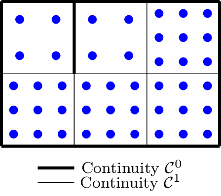
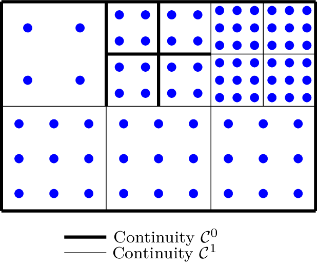
Once an appropriate refined Bézier mesh has been generated, the U-spline algorithm is applied to the Bézier mesh to generate the refined U-spline basis. These steps are shown in figure 137.
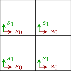
Figure 137b: A parameterized mesh which can be embedded in another mesh for one level of h-refinement.
Figure 137c: The final Bézier mesh resulting from embedding for one level of h-refinement. Local basis and continuity choices are made according to the simple method mentioned in Local basis and interface continuity requirements.
18.1.1.3 Projection of fields
Equipped with the base basis and the refined basis, geometry and simulation result fields represented in terms of the base basis must be transferred to the basis defined by the refined mesh. This is accomplished most easily by Bézier projection of the fields.
If we restrict our attention to nested spaces, then for each element in the embedded mesh , a matrix can be computed that transforms a function in the Bernstein form of the base element into the Bernstein form of the embedded element. Any field expressed in terms of the basis over the base mesh can be transformed to Bernstein form using the extraction operator. Once the Bernstein form in terms of the base Bernstein basis is obtained, the matrix can be used to perform a change of basis to the Bernstein basis over the embedded element: The local embedded Bernstein basis is identical to the refined Bernstein basis and so the Bernstein forms are equivalent. The refined Bernstein form is then projected to the refined basis using Bézier projection.
18.1.2 Local refinement
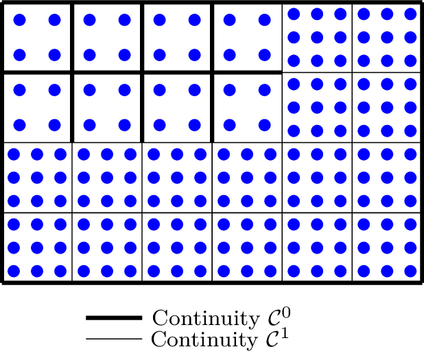
Local refinement can also be done through embedding. is simply embedded in a subset of the elements in instead of every element, which results in a topology that includes T-junctions. The local basis and continuity choices, the basis construction, and the field projection can proceed as in global refinement. A locally refined Bézier mesh is shown in figure 138.
Figure 138: The Bézier mesh resulting from one level of local refinement in the top left and top middle elements of the mesh shown in figure 137a. Local basis and continuity choices are made according to the simple method mentioned in Local basis and interface continuity requirements.
18.2 Hierarchical U-splines
A hierarchically refined spline is created from a series of nested globally refined bases. The basis meshes corresponding to these bases are created by globally refining the base mesh repeatedly until the highest level of local refinement desired is achieved. We will denote these refined meshes as and the parametric domain of these meshes (which is the same for each mesh) as . These successively refined meshes define a set of trees, with the elements forming the root nodes of the trees. We will focus here on dyadic refinement in a two-dimensional mesh, where the trees are commonly called quadrilateral trees or quadtrees, for short. The set of children of an element is defined as
and the natural extension to definitions of parent, ancestor, and descendant is employed. Each element is a node in one of the trees.
The hierarchical mesh is created from the globally refined meshes by specifying a set of leaf elements whose children will be pruned from the tree. The set of leaf elements is denoted as with , where is the parametric dimension. satisfies the following properties:
The elements are disjoint:
The elements cover the whole parametric domain:
We also define the set of elements which remain in the pruned trees as the active element set , where is the set of active elements on refinement level . can be computed from as
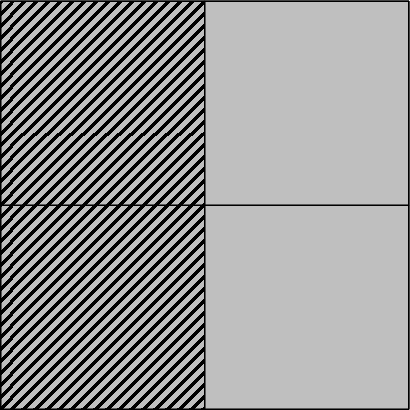
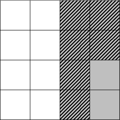
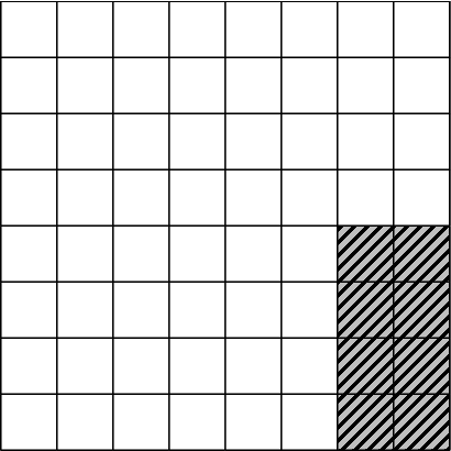
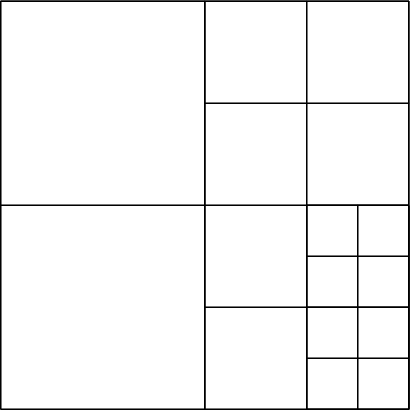
The parametric domain associated with each is defined as and these domains satisfy Example with and marked are shown for a three-level refinement in figure 139. Note that . During basis construction we make use of each of the separately, but once the basis is constructed, the final mesh presented to any downstream use of the basis is as if the local refinement desired had been performed as in Local refinement. This final mesh, which contains only the elements in , will be denoted as . The corresponding to the in figure 139 is shown in figure 140. The choices for refined local bases and continuity are made when constructing each , and need only satisfy the requirements for global refinement as outlined in Local basis and interface continuity requirements.
Figure 139: Example for a three-level refinement with active and leaf elements marked.
There are many considerations to make with regards to which elements to include in , including conditioning and number of degrees of freedom of the resulting basis, and approximation accuracy. These considerations will not be treated in this section, except to say that this hierarchical framework provides a general setting under which appropriate can be chosen.
Figure 140: Example for the three-level refinement outlined in figure 139.
18.2.1 Basis construction
The hierarchical basis over consists of basis functions constructed on each global refinement level. We will denote the U-spline basis on each as . These bases define associated spaces, which are nested, i.e., they satisfy
by construction of the . As such, any basis function in can be represented as a combination of basis functions in a higher refinement level:
The set of basis functions in which are also part of the hierarchical basis are called the active basis functions in the th refinement level, . This set is defined as
where . The union of these sets of active functions forms a basis over which we will denote as . In practice, the construction of a full basis on each refinement level is often unnecessary; constructing only over each is sufficient.
18.2.1.1 Core algorithm
Construction of only the active basis functions on each can be accomplished with a few adjustments to the U-spline basis construction algorithms outlined in The U-spline basis:
Instead of constructing a core graph from each 0-cell basis vector, we need only do it for the basis vectors .
If, during the core graph flood, a basis vector is added to the graph for which , terminate the flood and discard the result.
Once the active basis functions have been constructed on each , the basis vectors are rewritten in terms of the Bernstein bases on . For a truncated basis, however, more than just the active functions are required.
18.2.1.2 Truncation
The basis can be improved upon by discarding the contributions of finer active basis functions to coarser active basis function from those coarser functions. This process is referred to as truncation. Truncation improves the conditioning of the basis and gives it partition of unity. We define an operator which truncates a function with respect to the functions in refinement level as
The complete truncation of a function can be computed as
and the truncated basis is constructed as
In addition, we define the auxiliary function set of all functions truncated to level recursively as
where . Note that .
Truncation can be performed element-locally and level by level. Let the parametric region over which functions in are nonzero be denoted as
Let the set of functions in that touch functions in be denoted as
and the set of functions which are contained within the nonzero region of a coarser function as
We need to build the required basis functions on each to be able to represent all functions in over , namely With these basis functions built, we can can compute the element-locally by least-squares fitting the rows of the extraction operator to the Bernstein coefficients of the function to be truncated. The correct basis functions have been built to make the solution to the least squares problem exact even though the extraction operator may not be full rank.
18.2.1.3 Algorithms
◾ Recursively split and truncate function
1: procedure RecursivelyTruncate()
2: ▷ Construct or retrieve the splitting operator.
3: ▷ Split the expression to element .
4: ▷ Truncate the function.
5: if then▷ If the function has been truncated to zero on this element, we’re done.
6: return
7: end if
8: if then▷ If this is a leaf element, transfer the function to the hierarchical basis data structures.
9:
10: else
11: for each do
12: RecursivelyTruncate()
13: end for each
14: end if
15: end procedure
◾ Construct hierarchical basis
1: procedure BuildHierarchicalBasis
2: for each do▷ Loop over the refinement levels.
3: for each do▷ Process each active element in this refinement level.
4: if then
5: for each do
6:
7: end for each
8: else
9: for each do
10: for each do
11: RecursivelyTruncate()
12: end for each
13: end for each
14: end if
15: end for each
16: end for each
17: end procedure
18.3 Structured Hierarchical Splines
Hierarchical splines over structured regions can be efficiently assembled from the mass matrices for each refinement level, allowing us to take advantage of performant structured spline assembly routines in the hierarchical setting. This assembly is done using an operator, called the prolongation operator , which maps from the space of hierarchical basis coefficients to the direct sum of the spaces of refinement level basis coefficients. The transpose of this operator also expresses the hierarchical basis in terms of the refinement level bases. Hierarchical basis construction, then, can be seen as synonymous with creating . The prolongation operator can be built up level-by-level from refinement operators representing the global refinement of each level.
We first present some definitions to aid in the derivation. Let be the operator that, given a set of spline basis functions from refinement level , returns the indices associated with those functions in an index space . We define the matrix representing the active functions on a given level as a subset of columns of the identity matrix: We also define a refinement operator of size which transforms coefficients for level into coefficients for level . This operator may be created using the two-scale relation for uniform B-splines or by solving a linear system for the coefficients. See for example [81], which includes a discussion on these coefficients and how to obtain them.
The prolongation operator representing the truncated hierarchical basis can be built up level by level as follows: The prolongation operator is initialized from the active functions on level zero as and two other operators are initialized as , . For every level these operators are updated as and the prolongation operator is updated to include all active functions through level as Once the iteration has been performed for all refinement levels we have the final prolongation operator
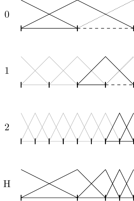
Consider the three-level hierarchical refinement over a two-element linear spline shown in figure 141. Derive the prolongation matrix using equation - equation .
Figure 141: Example construction of for a three-level refinement of a 1D linear basis. Leaf elements are indicated with solid black lines, active non-leaf elements with dashed black lines, and inactive elements with gray lines. Active functions are indicated with solid black lines, inactive functions supported only by active cells with dotted lines, and all other inactive functions with gray lines.
18.3.1 Mass matrix assembly
The mass matrix for the truncated hierarchical basis is constructed from the mass matrices of each global refinement level. Let the mass matrix for refinement level be denoted as . Also let , where products are performed by left multiplying. The mass matrix between all of the refinement level basis functions can be written as from which the truncated basis mass matrix can be assembled as
In most cases there will be many functions in each refinement level that do not interact with the truncated basis. We can further accelerate the assembly of by not assembling these functions. Let denote the block diagonal matrix and let We can then rewrite the assembly of the hierarchical mass matrix as By careful inspection of this last expression, we can determine that the only entries needed in are
While there are multiple possible that can express a given truncated hierarchical basis, we have chosen the above formulation because of the low number of nonzero rows in . Only the rows corresponding to active basis functions are nonzero, which means that less assembly is needed on the structured bases.
18.4 Simulations on hierarchical U-splines
In this section, we show a few examples of solid mechanics simulations on hierarchical U-splines constructed according to the above formulation.
18.4.1 Body-fitted plate with a hole
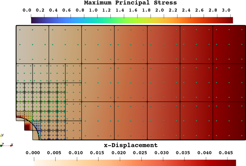
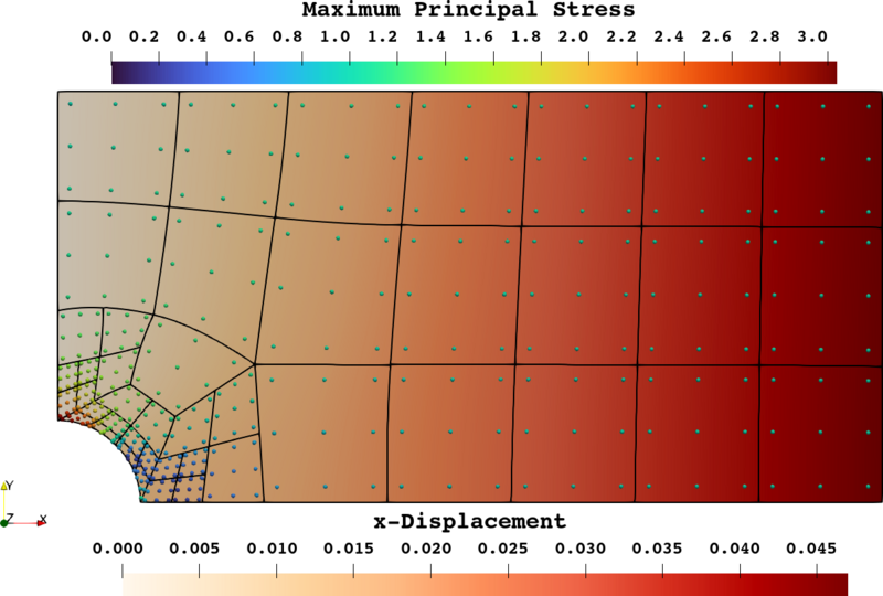
As a proof of concept, we ran a body-fitted simulation of a finite plate with a hole using a hierarchical U-spline. The plate was modeled as a quarter plate with symmetry boundary conditions on the bottom and left sides, and a constant pressure load on the right edge. The elements immediately surrounding the hole were refined two levels to better resolve the stress around the hole. Displacement and stress magnitude results are plotted in figure 142.
Figure 142: Results of a plate with a hole body-fitted simulation on a hierarchical U-spline. Displacement results are plotted over the elements, and stress results are plotted at the quadrature points.
18.4.2 Immersed plate with a hole
In addition to the body fit simulation, we also ran a proof of concept plate with a hole simulation in which the hole was immersed. The boundary conditions were of the same type as for the body fit simulation, and two levels of U-spline hierarchical refinement were performed to capture the behavior of the simulation in the vicinity of the immersed boundary. The results of this simulation are shown in figure 143.
Figure 143: Results of a plate with a hole immersed simulation on a hierarchical spline. Displacement results are plotted over the elements, and stress is plotted at the quadrature points.