8 Fitting
8.1 An Overview of CAD Fitting
We present a dimension-agnostic approach to fitting a -dimensional U-spline manifold to a -dimensional CAD manifold . Given an appropriate U-spline mesh , the core procedure consists of a local projection operation onto the corresponding Bézier mesh followed by the creation of a set of U-spline manifold control points through Bézier projection. The fitting operation is progressive, meaning the fitting workflow applies a manifold fitting sequentially for volumes, surfaces, curves, and points, overwriting manifold control point values from previous steps. The -manifold is first fit to , and submanifolds are defined over submeshes of dimension and fit to for each of the subsequent steps. These submeshes must be chosen such that the U-spline basis is linearly independent over the submesh. To accomplish this, the U-spline -manifold or for short is designed through the following process:
Step 1: A CAD model of the desired shape, denoted by , is created.
Step 2: CAD modification is performed as needed on to create . The CAD modification process is used both to eliminate dirty geometry in and to produce a topological layout that guides the mesh generation algorithm toward an optimal mesh for the U-spline basis construction and CAD fitting steps.
Step 3: A mesh generation algorithm is used to create a piecewise -linear approximation to , denoted by , where denotes the underlying mesh. The mesh provides the topology and a parametric domain for the construction of the U-spline basis and initial approximate CAD mapping . Numerous techniques are available for constructing . We focus on leveraging techniques widely available in standard finite element mesh generation software.
Step 4: We assume that is sufficiently well-defined that a closest point mapping can be constructed efficiently. This closest point mapping, denoted by , maps a given spatial point in to the closest point in . Given the mesh and the closest point mapping, we can define the following map This map provides an initial approximation to and a parameterization for U-spline fitting.
Step 5: A Bézier mesh is created from the mesh topology in . Cell domains, parameterizations, degrees, continuities, and Bernstein-like spaces are assigned to .
Step 6: The Bézier mesh is modified to create an admissible U-spline mesh and ensure that the resulting space is appropriate for the problem at hand.
Step 7: A U-spline manifold is created by fitting to the envelope CAD . A set of U-spline manifold coefficients (also called control points) is determined such that the resulting U-spline manifold mapping closely approximates , i.e., . The overall U-spline to CAD fitting workflow is dimension agnostic and includes a progressive approach, with sequential volume, surface, curve, and point fitting.
8.2 CAD Modification and Meshing for U-spline Surfaces
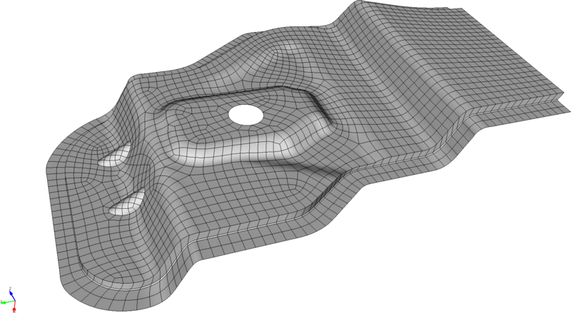
We demonstrate in figures 93, 97, 96, 95, and 94 an example of CAD modification and meshing for a simple CAD surface that results in a high-quality U-spline surface that closely approximates . As shown in figure 93, a CAD geometry representing a sheet metal automotive part is considered. As a first step, a highlighted surface associated with a blend feature is split producing a modified CAD object, denoted by , that will maximize the quality of the mesh. Additionally, a potentially troublesome sliver surface is identified immediately to the right of this surface. This sliver surface, if meshed in its current state, would require a very small mesh size and likely lead to poor mesh quality due to the small angle at its upper vertex. In figure 94, a surface-splitting operation is performed on the highlighted surface, decomposing it into two regions as shown in figure 94c. The top region retains a clear association with the blend feature while the lower smaller surface is now more clearly associated with the surfaces below the blend feature.
In figure 95, the surfaces associated with the fillet are composited into a single macrosurface (highlighted). This operation eliminates the problematic sliver surface but retains the geometric information provided by the surface. The meshing operation will enjoy increased robustness since it will only consume the composited surfaces during execution. As a final CAD modification step, eight additional macrosurfaces are created through compositing.
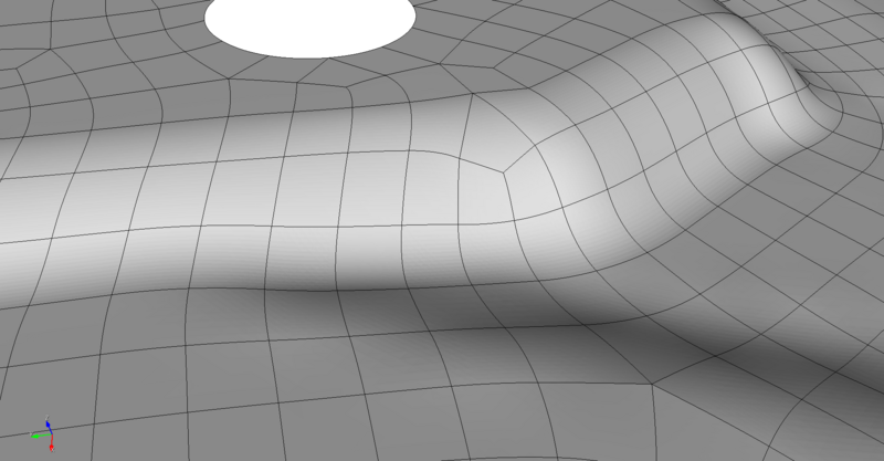
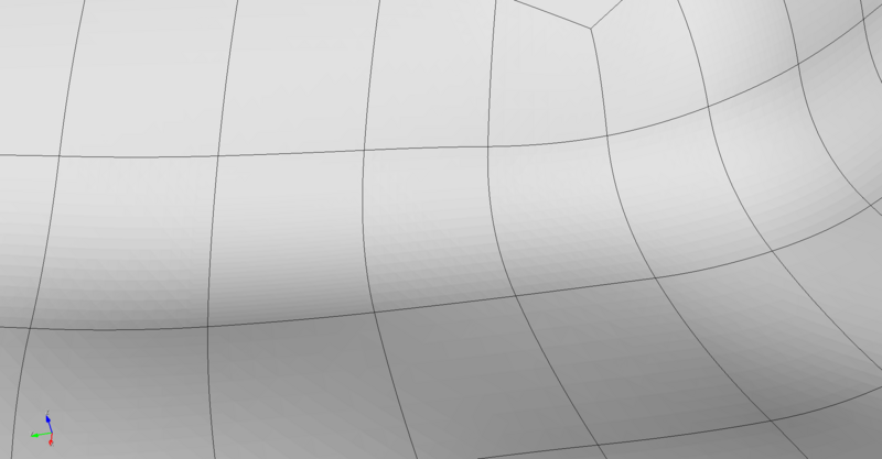
The modified CAD can now be meshed using any number of quadrilateral meshing schemes. In this example, an advancing front meshing algorithm called paving is used. The resulting mesh, denoted by and shown in figure 96, respects the topological layout produced by the macrosurfaces created previously and is of high quality. As described in the following sections and shown in figure 97, the mesh can then be converted into a U-spline.
Figure 93: A midsurface CAD geometry representing a sheet metal automotive component that will be converted into a U-spline.
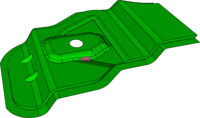
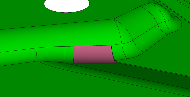
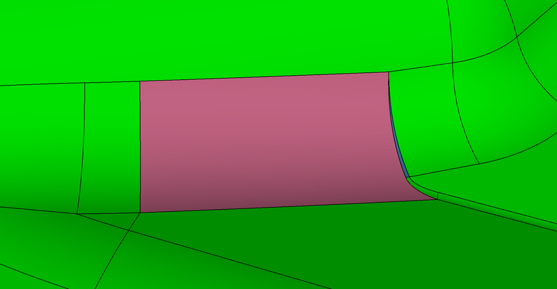
Figure 94: The highlighted surface is split into two surfaces that provide a more consistent representation of the blend feature.


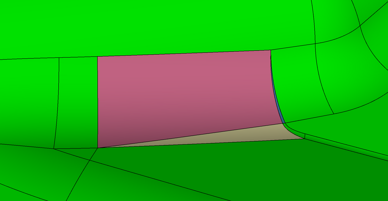
Figure 95: The CAD is further modified by compositing CAD surfaces into macrosurfaces. The macrosurface layout guides the mesh generation algorithm to produce a high quality quadrilateral mesh.
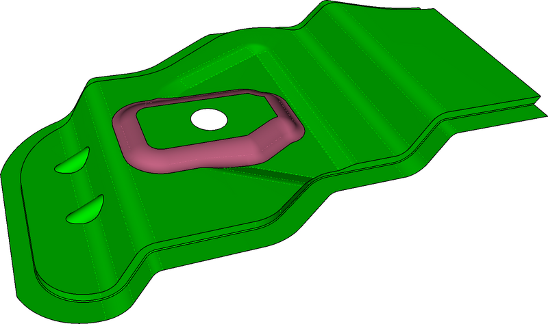
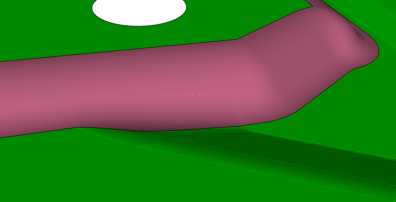
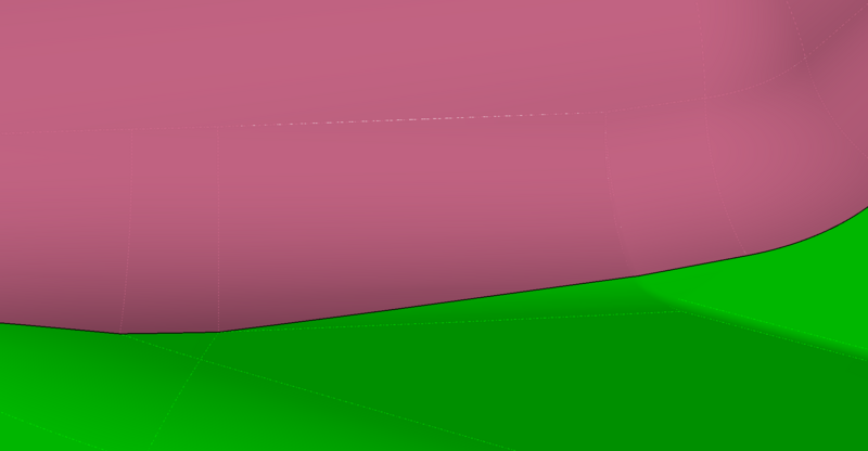
Figure 96: The geometry is meshed. The blend feature is accurately captured by the mesh.
8.3 CAD Modification and Meshing for U-spline Volumes
The CAD modification and meshing procedure to create a U-spline volume is more complex than for surfaces. This is because the interior of must also be filled with a mesh and, to maximize the benefit of the U-spline basis, the mesh should be a high-quality hexahedral mesh. High-quality hexahedral meshes as input into the U-spline basis construction process result in efficient, accurate, and robust simulation models.
The current state-of-the-art in hexahedral mesh generation is to decompose the BREP into simpler subdomains and then mesh each subdomain individually with a semi-structured hexahedral mesh generation scheme. To facilitate recombining the subdomains after meshing, an imprint and merge step is performed which ensures that adjacent subdomains share common BREP topology. This imprinted topology is leveraged by the hexahedral mesh generation algorithms to ensure the resulting mesh is conforming or, in other words, that no hanging nodes or T-junctions are present in .
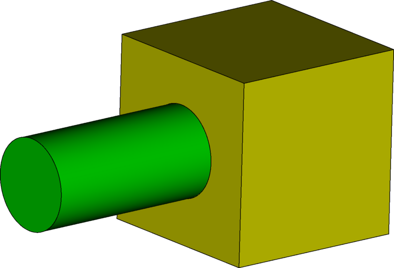
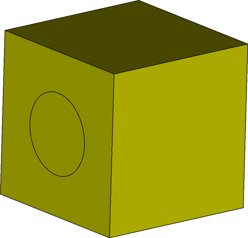
This decompose, imprint, and merge process is shown in figure 98. After a decomposition step (see figure 98a), two disconnected BREP volumes are created that do not share any topological information. A non-conforming (i.e., mismatched) hexahedral mesh is created (see figure 98b) if the imprint and merge steps are not performed. Imprinting and merging the geometry across the interface (see figure 98c) adds the cylinder BREP topology to the cube face. The duplicate surfaces are then merged resulting in two BREP volumes with matching topology. A conforming hexahedral mesh can then be created (see figure 98d).


Once a BREP is decomposed into simpler subdomains a (semi) structured hexahedral mesh generation scheme can be applied to each domain. The workhorse algorithms are usually based on a tensor product or mapped mesh generation algorithm or a sweeping mesh generation algorithm where an unstructured quadrilateral mesh is swept along a curve defined by adjacent linking surfaces. Other, more sophisticated hexahedral mesh generation schemes exist but are usually a combination of these simple approaches. The hexahedral mesh can then be converted into a U-spline volume and fit to the original CAD model such that .
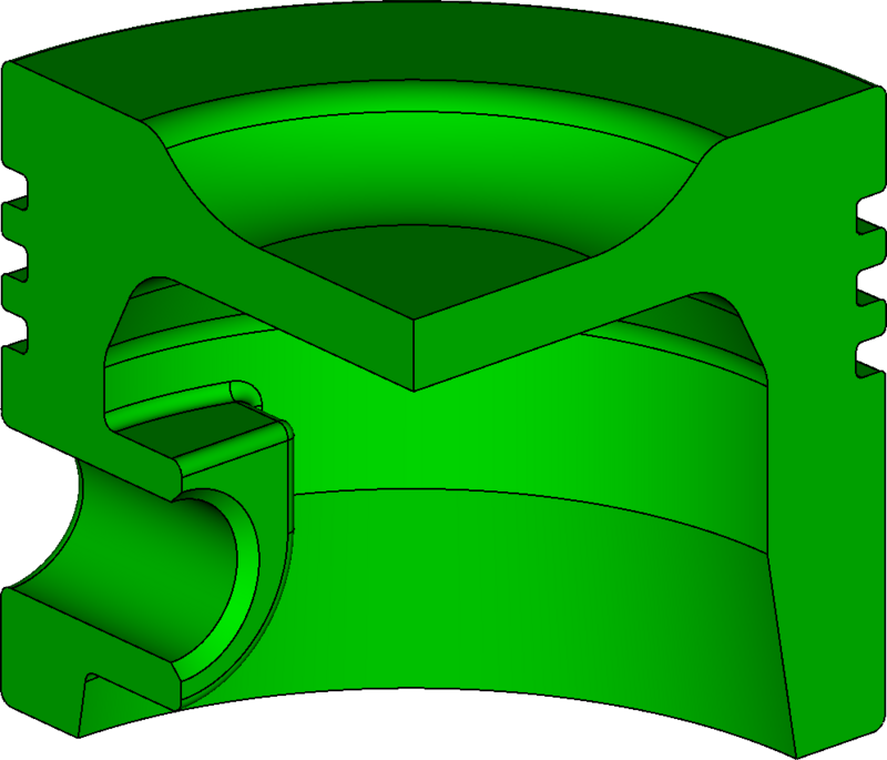
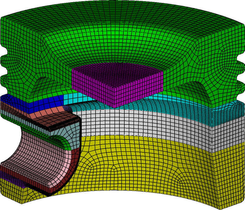
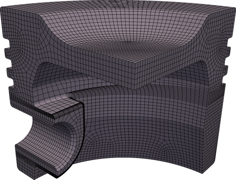
This process applied to a BREP CAD model of a piston is shown in figure 99a and figure 99c. Notice that the piston CAD model is decomposed into multiple subdomains each of which is swept to produce the final conforming hexahedral mesh. The resulting U-spline volume smoothly and accurately captures the features of the original CAD model .
Figure 99: The process of converting a CAD volume into a U-spline volume leveraging CAD modification and hexahedral mesh generation.
8.4 Unstructured U-spline CAD Fitting
Unstructured CAD fitting leverages a progressive fitting approach as follows:
Calculate an approximate using -manifold fitting based on Bézier projection as described in U-spline Geometry.
- For each
Choose an appropriate -dimensional submesh .
Calculate a partial set of manifold coefficients over using -manifold fitting as descrbed in Submanifold Fitting.
Overwrite the corresponding coefficients from the previous steps.
The expansion of the U-spline basis with the resulting coefficients is denoted as .
The submeshes are typically chosen to include cells on the boundary or along features of interest, so long as the U-spline basis is locally linearly independent over those cells.
8.4.1 Submanifold Fitting
The approximation of provided by can be further improved using submanifold fitting. While the application of Bézier projection to alone does give an approximation of , it does so considering only the interiors of each element. As such, the approximation is typically poor at the boundaries of the manifold. This can be mitigated by fitting a series of -manifolds defined over boundary submeshes . The submanifold fits only consider the boundaries, and will therefore match them more precisely.
Submanifold fitting proceeds much as -manifold fitting. Once an appropriate -dimensional submesh has been chosen over which the U-spline basis is locally linearly independent, we first project into the Bernstein space assigned to each -cell in . We then compute for each cell as This piecewise discontinuous approximation is then converted to a partial set of U-spline coefficients by averaging the results of Bézier projection on each submesh cell, computed as
Progressive fitting algorithms can make use of these boundary coefficients in a variety of ways. Coefficients calculated in the interior fitting can simply be overwritten by the boundary coefficients, or the boundary coefficients can be used as constraints for a smoothing adjustment of the interior coefficients.
8.5 Structured U-spline CAD Fitting
The fitting routines presented in Unstructured U-spline CAD Fitting assume no structure in , , or . If some structure is present in the U-spline basis and geometric mapping, algorithms can be developed that are orders of magnitude more performant than the general unstructured routines. We assume in this section that is a -manifold embedded in .
8.5.1 Tensor Product Fitting
We say is tensor product if there exist bases such that where , and . Note that a scalar indexing for functions in can be obtained from the vector indexing as We begin each structured fitting routine by fitting to to produce . These fits can be performed using Bézier projection as described in Unstructured U-spline CAD Fitting. We present these tensor product manifold fitting routines in order from most to least structured.
8.5.1.1 Affine Fitting
If is an affine transformation of a -cube, that transformation can be described as the combination of a linear transformation and a translation . Control points in can be calculated by performing this transformation on the direct sum of control points from . In other words, where , , , and follow the conventions above. and can easily be calculated from the corner coordinates of . This fitting method requires the storage of floating point values, which encode , , and each .
8.5.1.2 -linear Fitting
If is a -linear cube, the control points can be calculated as a -linear interpolation of the corner coordinates. We denote -linear interpolation between the corners of as . Control points in can then be calculated as where , , , and follow the conventions above. If is an affine transformation of a cube, this fitting method will produce the same results as that in Affine Fitting. This fitting method requires the storage of floating point values, which encode the corner coordinates of and each .
8.5.1.3 Coons Patch Fitting
Coons patch fitting takes a fit of the entire boundary of and interpolates it to the interior. There is no geometric structure required for Coons patch fitting, though there are extreme cases where it may fail to produce an appropriate parameterization. In these cases the fitting may fall to the algorithm described in Unstructured U-spline CAD Fitting.
Coons patch fitting can be formulated as follows:
We first define a series of bases , where , as where is a tuple containing for . is taken to be a point basis with one function, . For convenience we also define . Note also that is the restriction of to any one of the submeshes for which . We denote these submeshes as , where is a tuple containing 0 or 1 for each . A boundary fit for also defines coefficients for each and associated -manifolds. Therefore for each pair there are coefficients given by the choices for , where contains the th components of for .
We now define to be the -linear interpolation between the set of . We also define the tuple Coons patch construction can be written as a combination of several of these interpolations, i.e.,
Coons patch fitting requires the storage of floating point values to encode each , as well as whatever storage is used for the boundary fit. If is a -linear cube, this fitting method will produce the same results as that in -linear Fitting.
8.5.2 Composite Fitting
For less structured where every cell is cube-like, such as multi-patch NURBS or swept meshes, can be decomposed into the union of some number of structured regions, and can be expressed as a linear combination of tensor product bases. is then termed a composite function space, or a composite basis, and the structured subregions are called patches, with associated function spaces . When this structure is available, it is possible to take advantage of the structure in the patches to obtain a fit to in a much more performant manner than using unstructured fitting routines.
A composite function space , stored with the structure intact, has a global extraction operator that stores the linear combination coefficients expressing elements of in terms of elements of .
The composite fitting procedure is composed of three steps. First, the composite Bézier mesh is constructed. Second, the prolongation operator is constructed. The prolongation operator transforms a set of U-spline manifold coefficients into the direct sum of coefficients for each structured submanifold. Third, the restriction operator , which satisfies , is constructed. The restriction operator expresses the manifold coefficients for the composite manifold in terms of the coefficients for the structured submanifolds, allowing us to compute the U-spline manifold coefficients given submanifold fits for each structured patch.
8.5.2.1 Constructing the Composite Bézier Mesh
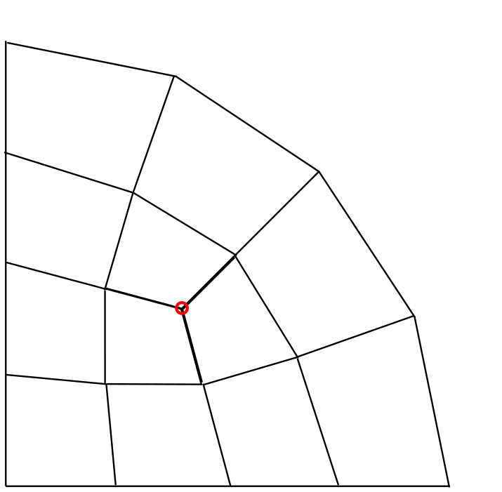
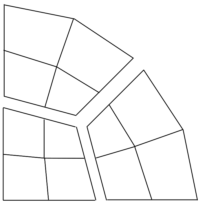
The first step in building the composite function space is to build the composite topology and Bézier mesh. This is done by first creating the motorcycle graph following Eppstein et al. [32]. An example of this is shown in figure 100.
Figure 100: (a) An unstructured quadrilateral mesh of a quarter circle. The red circle highlights a valence three extraordinary point. (b) The unstructured topology decomposed into three tensor product topologies. These constitute the subtopologies of the resulting composite topology.
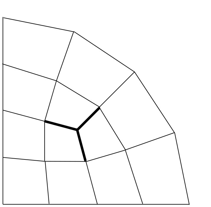
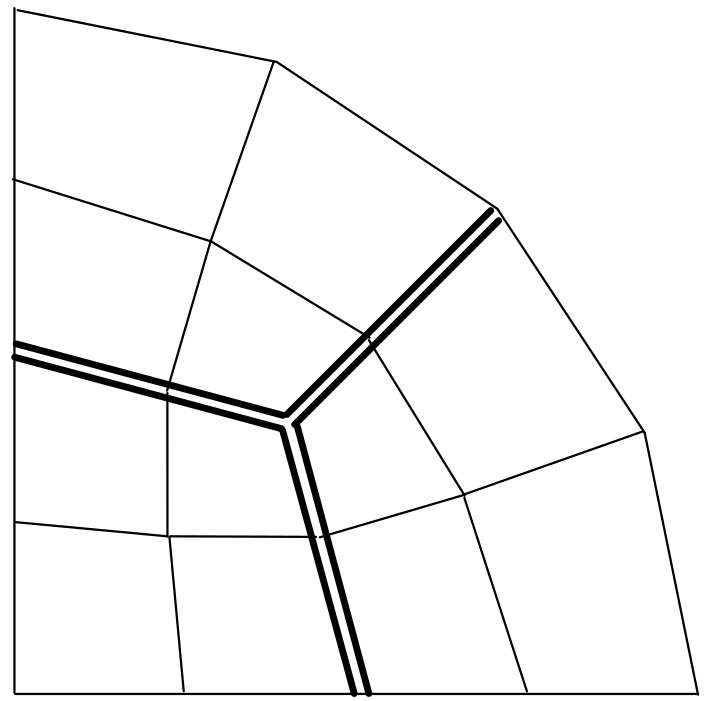
Once the composite topology has been created, a composite parameterization is created by assigning all edges a parametric length of one. We next create two Bézier meshes over the parametric domain. The smooth Bézier mesh is created by assigning a global default degree and continuity for the Bézier mesh. Then, interfaces in the mesh are creased to ensure an admissable Bézier mesh is generated. Then, the structured Bézier mesh is constructed by assigning a default degree and continuity to each structured subparameterization. Then, the interfaces between subparameterizations are assigned continuity. Finally, we can construct the set of smooth U-spline functions over the smooth Bézier mesh and the set of B-spline basis functions over the structured Bézier mesh. An example composite layout is shown in figure 101.
Figure 101: The two Bézier meshes needed to construct a composite U-spline. All elements are Bézier elements. Thin lines denote continuous edges, thick lines denote edges, and thick double lines denote edges. (a) The smooth Bézier mesh. (b) The structured Bézier mesh.
8.5.2.2 Constructing the Prolongation Operator
Let denote the global Bézier reconstruction operator for the set of NURBS basis functions. Let denote the global extraction operator for the U-spline basis functions. The prolongation operator can now be calculated using Bézier projection as
8.5.2.3 Constructing the Restriction Operator
Typically, we will construct the operator from the operator . The operator is not unique. One potential choice is the pseudoinverse of but in general this will not be sparse and so is poorly suited to use here.
We seek an operator with a minimum number of nonzero entries. One convenient approach draws inspiration from Bézier projection. We will construct each row of the operator separately using a subset of the columns in the operator. Let the operator return the set of indices for nonzero entries in a row or column vector. Let represent the set of row indices associated with a single function: . Let represent the set of indicies satisfying For now, we assume that . If this is not the case then we will need to introduce additional steps. With this assumption, we assume that the nonzero entries of the th row of have the same indices as the nonzero entries of the th column of .
We assume the existence of an operation that assigns a unique number from a consecutive sequence (typically starting at 1) to each element of a set. We call this the enumeration operation and denote it by .
If then the entry corresponding to the single index in the th row of is one. We can cast the requirements for the nonzero entries of the th row of in matrix form by defining where and . Let the vector be the vector containing the nonzero entries of the th row of : where . The requirement that can be separated into two parts: products that are equal to zero and products that are equal to 1. The first requirement can be expressed as Recall that the matrix contains only the entries associated with the columns whose nonzero entries overlap with the th column but does not include the th column.
The second requirement on the entries of the th row of is that
This requirement can be expressed several ways, each of which produces a different result. The simplest method to impose this constraint is to augment the linear system
This has the result of averaging all contributions to the final value evenly.
An alternative is to weight the contributions from different patches according to their relative weight. We introduce the patchwise weight coefficient where is the patch index. This represents the relative contribution of each patch to the th function. By construction, We also define the vector with entries
Every column index in the matrix coresponds to a global function. Every row index in the matrix corresponds to a local function in a patch or subdomain. A function can be constructed that maps a row index to the associated patch index. We also require a function that maps a function index to the set of subdomain indices on which the function is supported. We use to refer to this subdomain support function. We define the matrix, , having one row for every patch on which the th function has support. The nonzero entries of are where and . With these definitions, we arrive at the linear system of relationships that define one row in :
Depending on the dimensions and other requirements, this can be solved by linear programming or using a pseudoinverse.
8.6 Improving CAD Fitting Through Local Smoothing
It is possible for the progressive fitting algorithm above to produce inverted manifold elements if there is enough discrepancy between the interior and boundary fits. This typically occurs for a -manifold in a -dimensional space when the mesh is rather coarse compared to features of .
While this issue can sometimes be avoided with a better mesh, we can improve the robustness of the fitting routine by adding a coefficient smoothing step. This smoothing step, instead of just overwriting the coefficients from the higher dimension manifold fits, uses the boundary fit as boundary conditions for a Laplace solve, thus adjusting the interior coefficients as well as the boundary coefficients.
We first detect elements that may be inverted. Detection may be done by calculating the higher-order Jacobian determinant, but this can become prohibitively expensive and typically requires a dense sampling scheme to accurately detect inversions. We adopt the approach of checking the Bézier control nets on each element for inversions. While this is neither a sufficient nor a necessary condition for inverted manifold elements, it is sufficient in nearly every case, and is quick to compute.
The domain over which we apply the smoothing operation includes the elements with inverted Bézier control nets as well as any elements within adjacencies of those elements. In other words, let the set of elements with inverted Bézier control nets be denoted as .
We define a recursive adjacency operator such that and We futher extend the definition of to sets of elements as
Then, the submesh over which smoothing is applied is for some .
We smooth the manifold coefficients using a Laplace smoothing step. To simplify notation, we assume and use to denote the volume we want to smooth and to indicate the surface computed during a prior progressive fitting step. We will use to define the displacement boundary condition for the Laplace smoothing of .
The strong form of the problem can be stated as: find such that We use Coreform IGA to compute the solution to this problem. The displacement solution coefficients are added to the U-spline coefficients of to determine the smoothed U-spline.
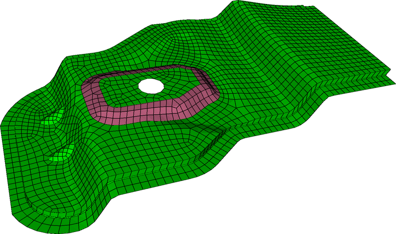
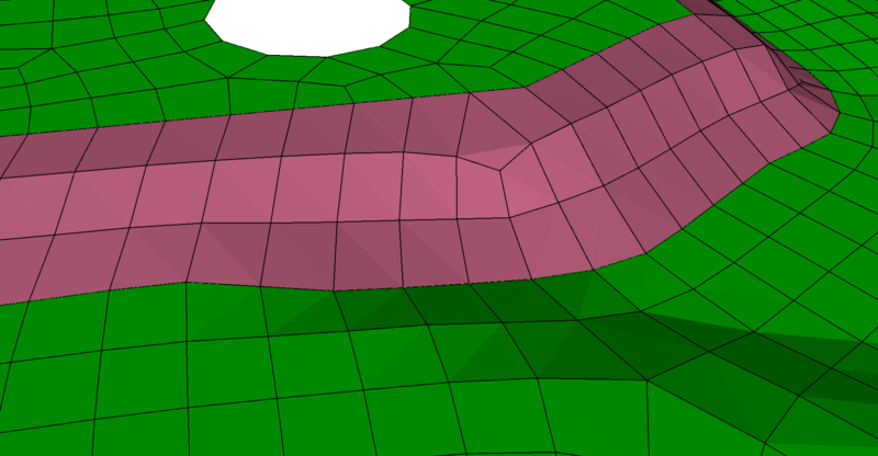
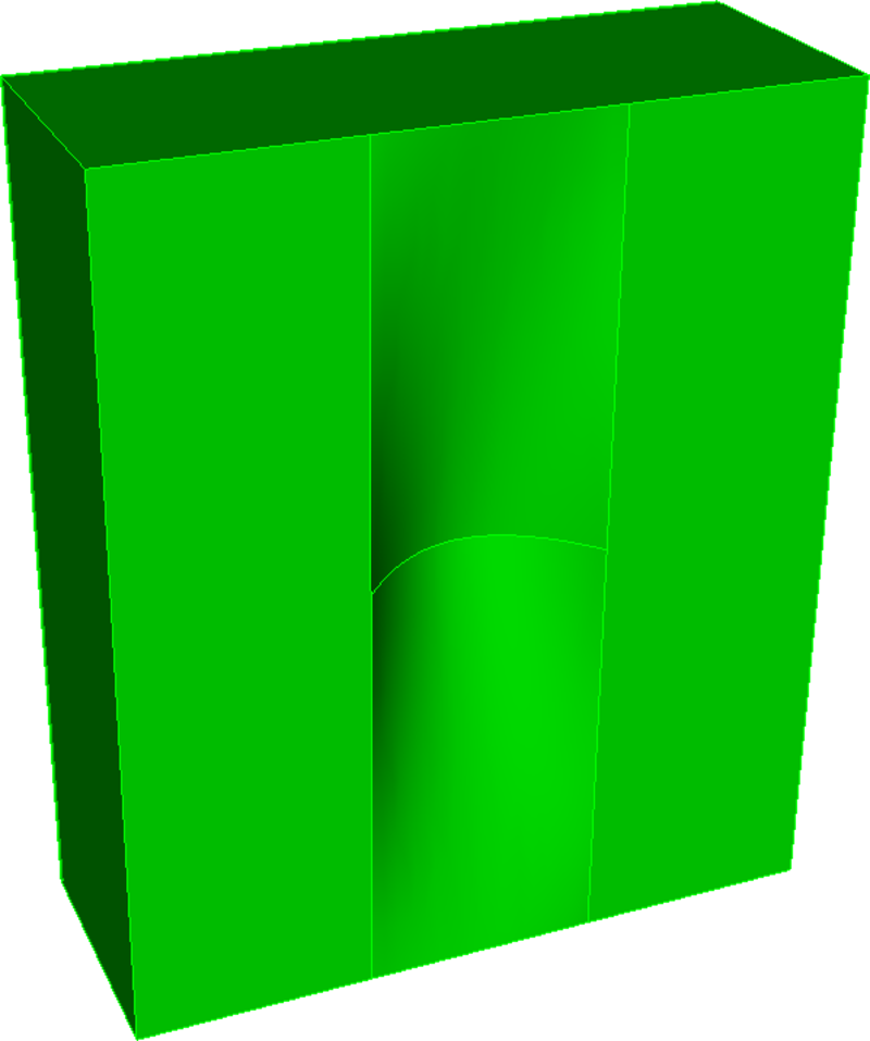
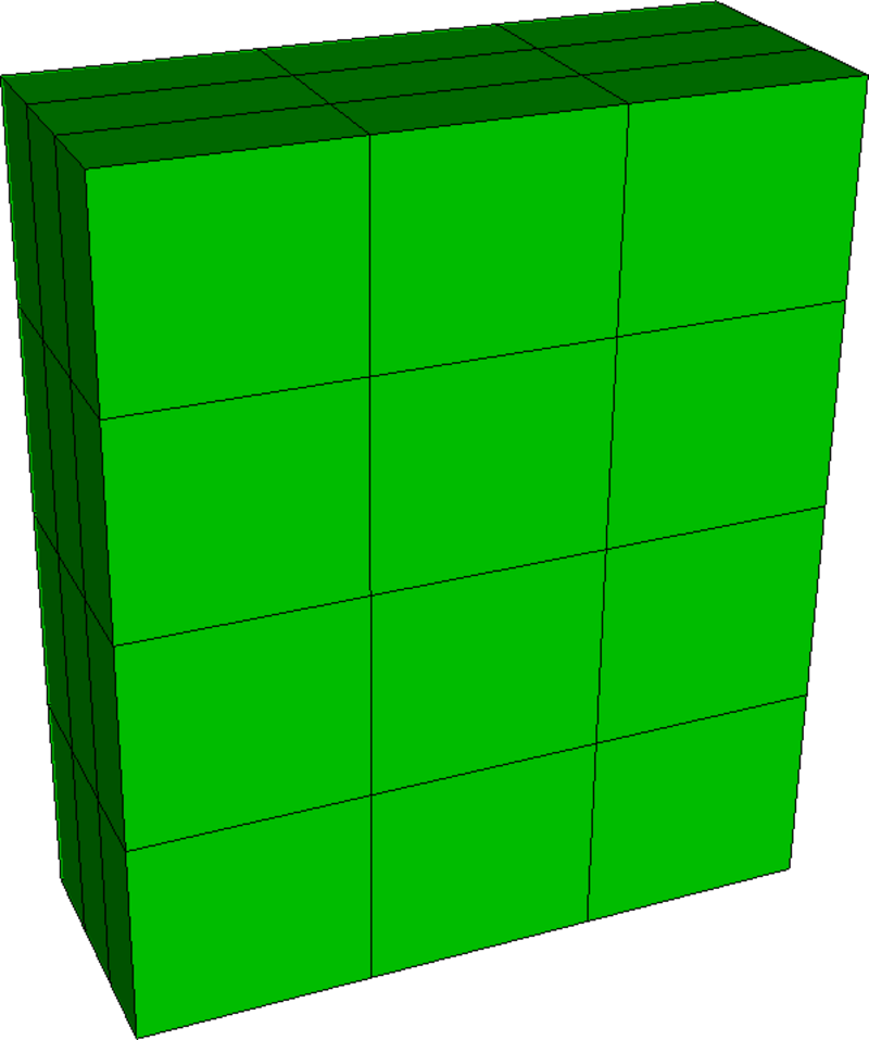
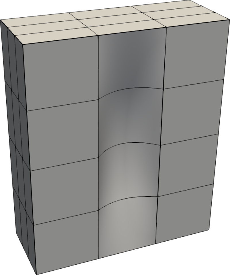
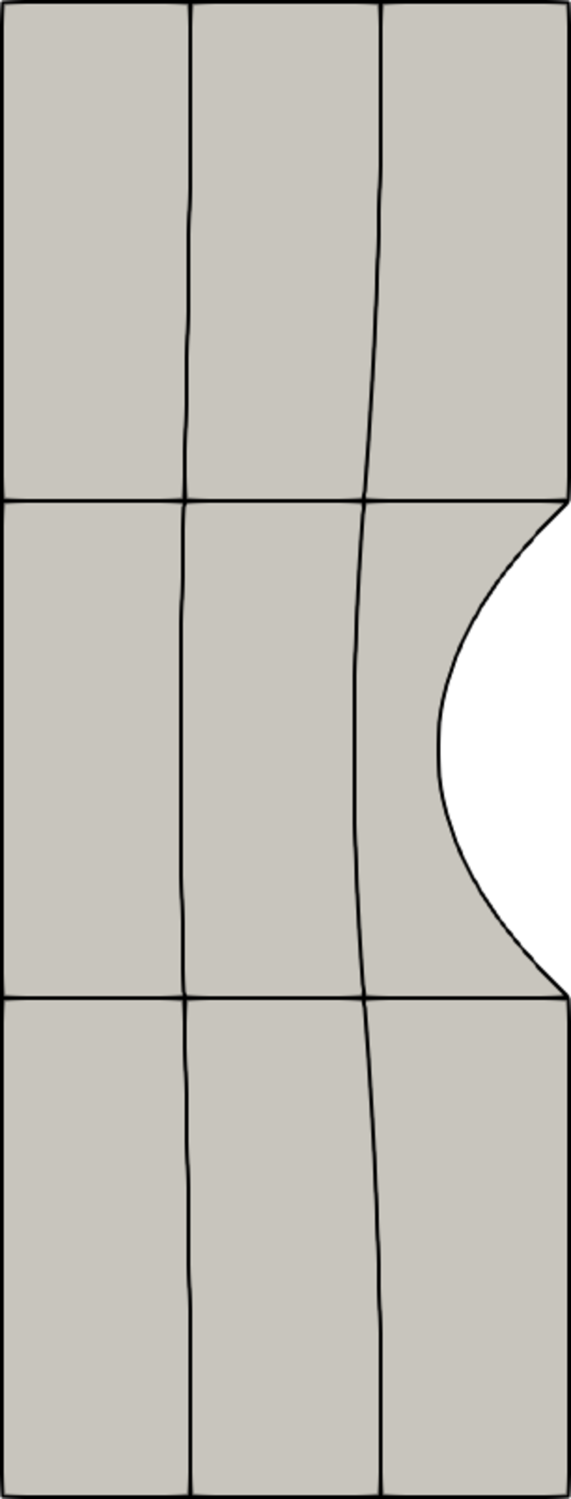
We demonstrate smoothing fitting on a simple example. In figure 102a is pictured a which is a brick with a curved divot taken out of it. This CAD is meshed with the poor mesh shown in figure 102b. While the linear approximation given by completely ignores the divot in the original CAD, the created by fitting a quadratic U-spline with the smoothing fitting (shown in figure 102c) is able to recreate the divot.
Figure 102: An example of a volumetric manifold fitting for which smoothing is necessary.
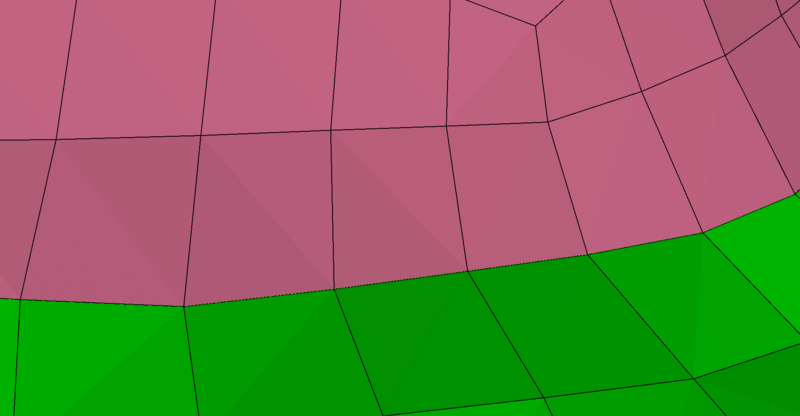
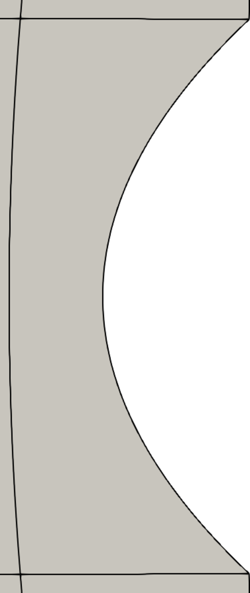
The smoothing operation is necessary in this case in order to avoid inverted elements. Figure 103 shows the cross section of fit with the progressive fitting scheme, i.e., without any smoothing. In the detail shown in figure 103b, we see inversion of the element. This is due to a mismatch between the interior and the boundary fitting coefficients. If instead we apply the smoothing fitting scheme, we get the results shown in figure 104, where element inversion is no longer present.
Figure 103: A cross-sectional view of fit with the progressive fitting scheme.
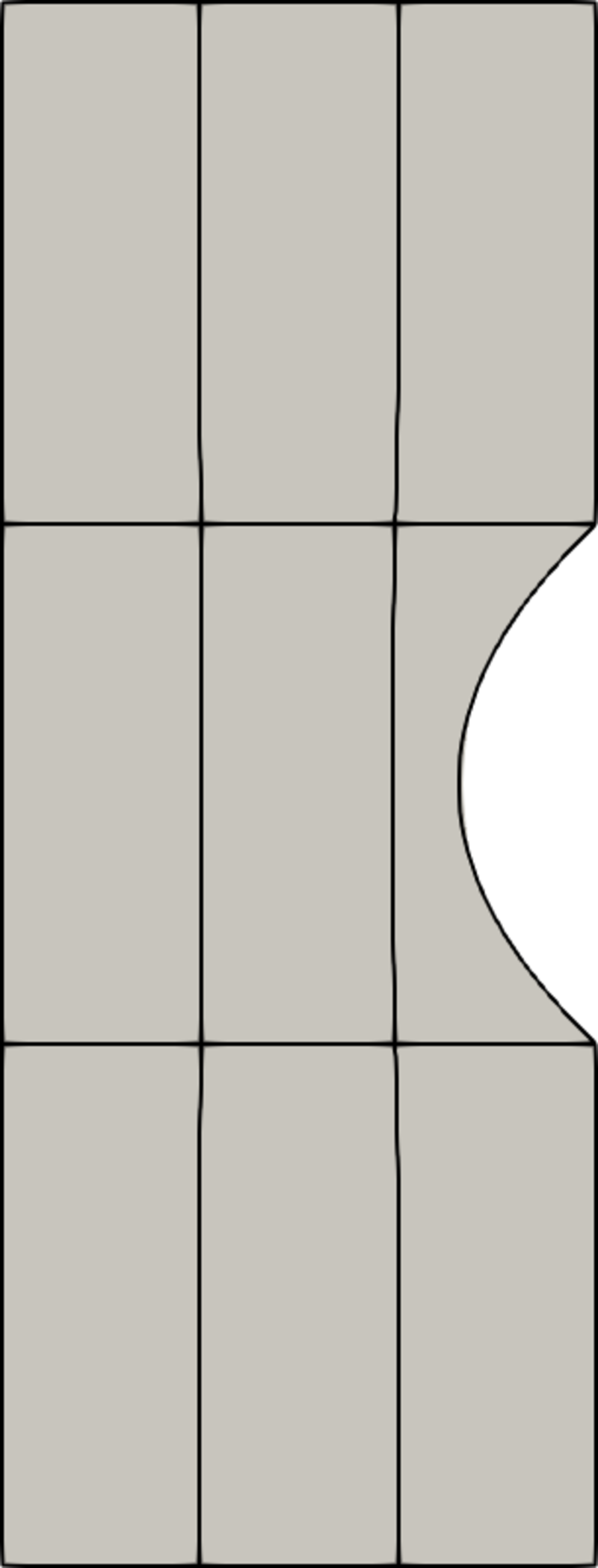
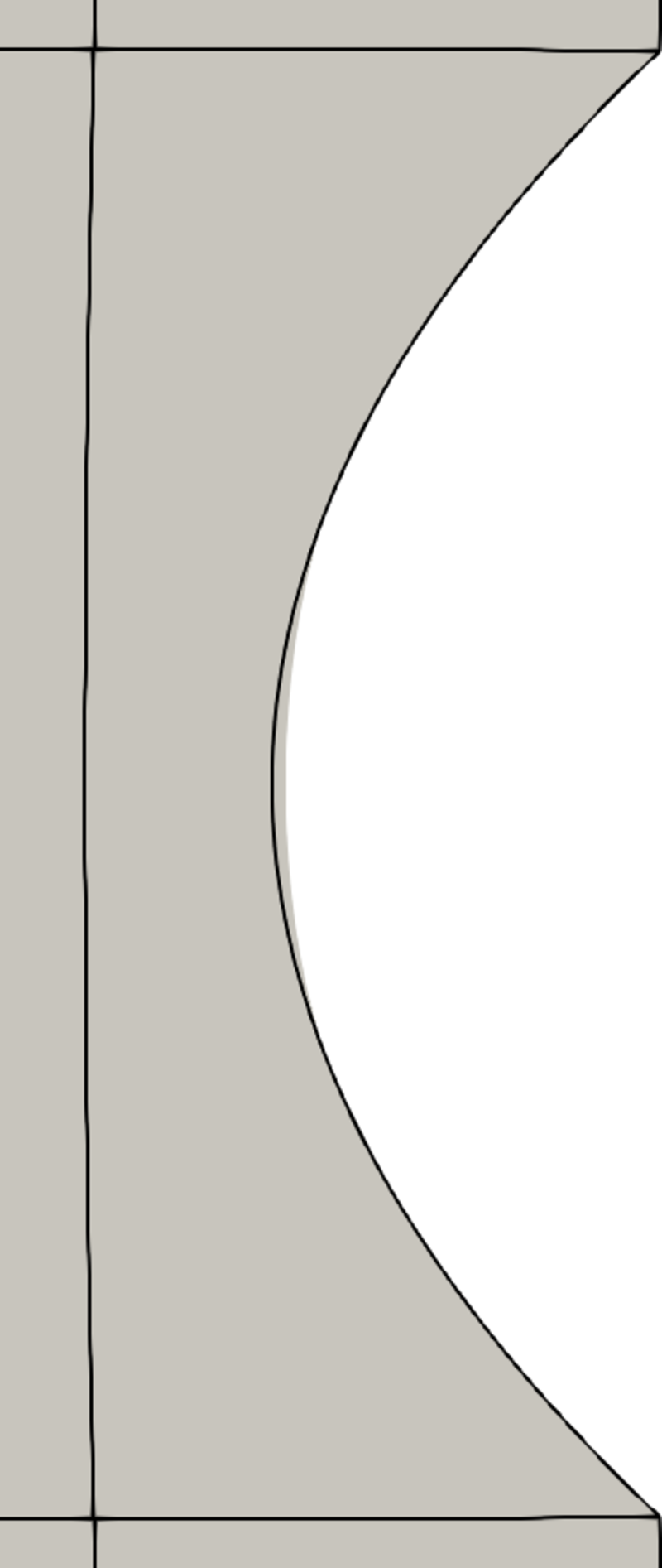
Figure 104: A cross-sectional view of fit with the smoothing fitting scheme.
8.7 U-spline CAD Fitting Examples
We demonstrate the effectiveness of the U-spline to CAD fitting process on several surface and volume problems.
8.7.1 Surface Fitting
Figure 105 shows a U-spline that captures the sharp corners in the CAD geometry.
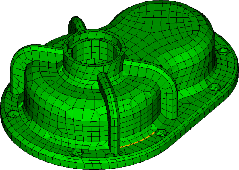
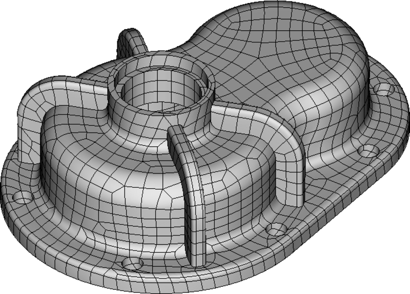
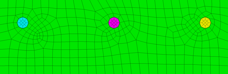
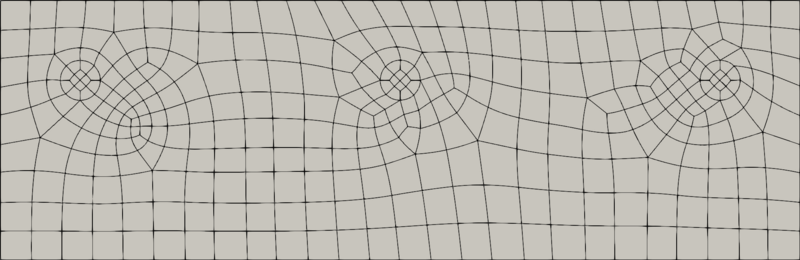
Figure 106 shows a U-spline fit to a planar surface that includes circular features. To resolve the circular features, a curve fitting is applied to the manifold edges of the circular features after the surface projection is applied.
Figure 106: Applying surface and curve fitting to a planar surface with circular features.
8.7.2 Volume Fitting
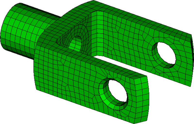
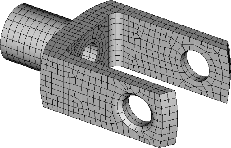
Figures 107a, 107b, 108a, and 108b illustrate the behavior of the U-spline to CAD fitting algorithm for U-spline volumes. As expected, high-quality approximations to the original CAD models is achieved in both cases.
Figure 107: Fitting a quadratic U-spline volume to a spinal implant model
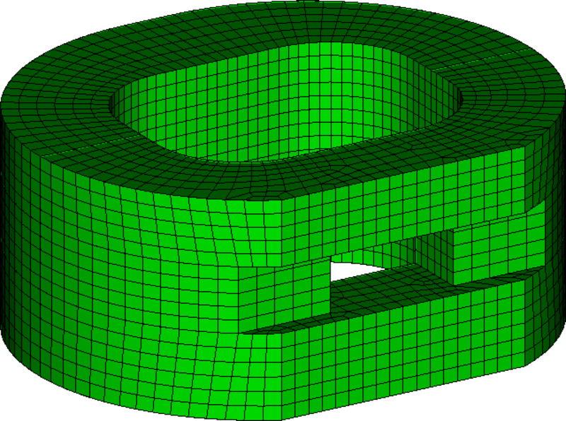
Figure 108: Fitting a quadratic U-spline volume to a knuckle geometry.