11 Basis Conditioning
11.1 An Overview of Basis Extension
The trimmed U-spline mesh may contain sliver elements that, if left untreated, can lead to poor conditioning of the U-spline basis when used in numerical procedures. The basis conditioning process detailed here is a way to systematically eliminate the impact of small sliver elements on the U-spline basis thus improving the conditioning of the basis. The main idea is to remove the basis functions that are only supported by small elements and then smoothly extend the remaining basis function supported by the larger elements to the small elements using weighted combinations of the basis functions defined over the large elements. The method described here is based on [16].
Partition the elements in into small and large elements based on a classification parameter .
Form an association between small and large elements.
Create a local extension operator for each association.
Assemble the global extension operator as the weighted sum of the local extension operators.
11.2 Element Classification
We define the set of small elements, , as and the set of large elements, as where are the elements in the U-spline that are trimmed or cut by the trimming surface .
In the case where the every element is a cut element we scale the partitioning parameter as Where and is the initial classification parameter.
11.3 Element Associations
The set of interfaces adjacent to an element, , of dimension is given by . In the presence of a trimming surface, the measure of the portion of the interface, , interior to the trimming surface, is used to determine associations of adjacent elements in the construction of the extension operator. We use to represent the interface adjacent to with the largest interior measure: where If multiple elements have interior measure equivalent to the max then the choice is arbitrary. We often choose the interface with the smallest identifier.
The set of all elements that neighbor the element is given by . We will define the maximal neighbor of an element as
11.3.1 Association Generations
We introduce a partitioning of the set of small cells into disjoint subsets known as generations. We use the symbol to represent the th generation and adopt the convention that the root generation . The relationships between these subsets is inferred from the maximal interfaces. We define the th generation as
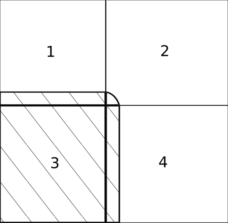
A simple example with numbered elements is shown in figure 113. In this example, , , and .
Figure 113: An example with multiple association generations.
11.4 Association Extension Operator
The construction of extension operators begins with the definition of a transformation between bases at the Bernstein level. We wish to to construct a relationship between the functions supported on large elements and the functions supported on small elements. We begin with two adjacent elements, and . We assume that we have a function space, , of dimension that is defined over both elements. Let the sets of indices of the functions supported on and be represented by and , respectively. We will employ the scatter operators and that map coefficients indexed with respect to the local basis used to define the extraction operators into the vector of coefficients of the global basis associated with . We assume that we are given affine embeddings and where is the parametric dimension of the elements. Let be a (typically polynomial) function space over such that for any function , and for any function , . We can define change of basis operators, and , that transform the representation of functions from the element-local bases to the shared basis: and A function over can be transformed or extended into a function over as
We assume that we are also given transformations that provide representations of the basis for the global function space, , over the elements and as linear combinations of the bases and : and These are known as element extraction operators. We combine the element-to-element transformation defined previously with the element extraction operators to define a transformation from global spline coefficients on to global spline coefficients on : We will take to be an element in and to be which is a member of .
In order to combine the element extension operators into a global extension operator we will also require the measure of each element and the measure of all elements in the intersection of the support of a single function with the trimmed region. For each element we can define a local weighting matrix where is the th member of the set of functions supported on the element .
We define the generation index set, as the set containing the indices of all functions support on elements that are part of the th generation but not part of any previous generations. We also define the cumulative generation set as the union of all preceeding generation index sets:
With these definitions the extension operator is defined as a weighted summation where is the set of function with support on and is the set of functions with support on . The full extension operator is defined as the composition of the extension operators from each generation: where is the number of generations. Note that by definition is the identity matrix.
11.5 Initial conditions with basis extension
Initial conditions are always defined on the extended basis. We need a way to determine the initial condition coefficients for the compressed basis.
Let represent the the extended set of initial condition coefficients and represent compressed set of initial condition coefficients.
where , and are the basis functions. Similarly, where is the global extension operator.
We minimize the difference between the extended initial conditions, which are known, and the compressed initial conditions which are not known.
Given the conventional norm on , this can be written as
We minimize by taking the partial derivative with respect to the compressed initial condidition coefficents and setting the resulting function equal to 0.
After the product rule
Rearranging and expanding
Let , we can reduce to a matrix equation
11.6 Effects of basis conditioning on stress
To quantify the effects that basis extension has on stress we run a series of patch tests with and without extension enabled and compare stress values in the areas of small elements.
11.6.1 Simple cube patch test
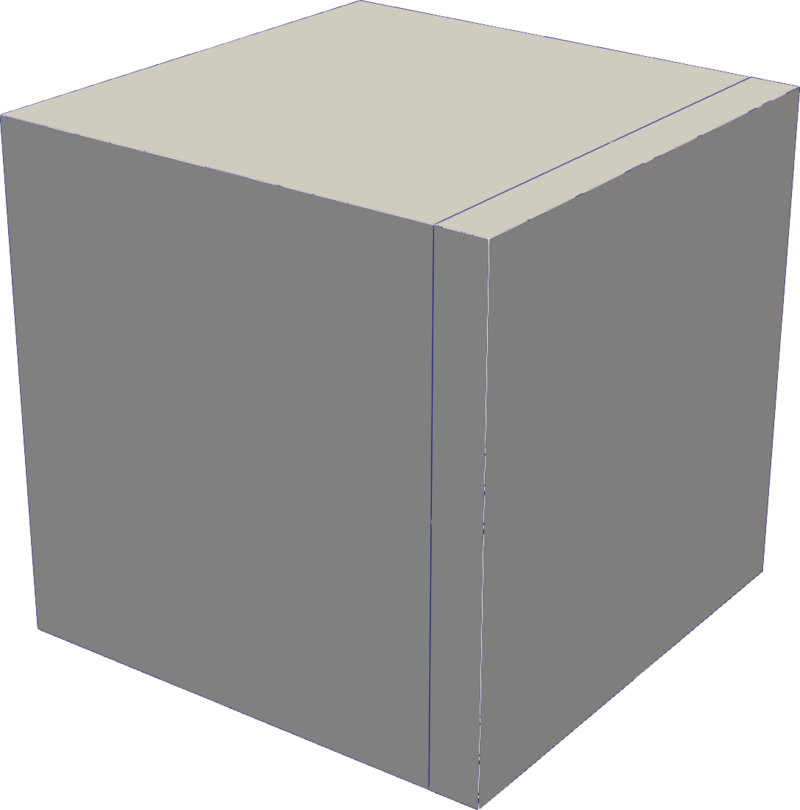
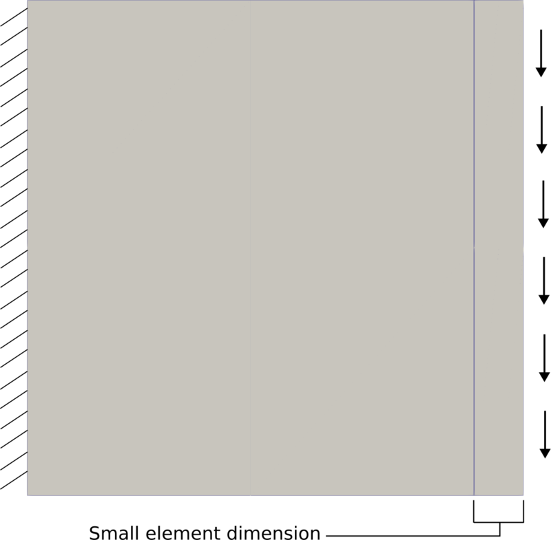
This test is a simple 1 x 1 x cube that is partitioned into a large cell cell and a small cell by a planar surface.
We hold the constrain one face to have 0 displacement in all directions and constrain the opposite face to move in the X direction.
Extremum probes are used to measure the value and location of highest stress values in each principal direction.
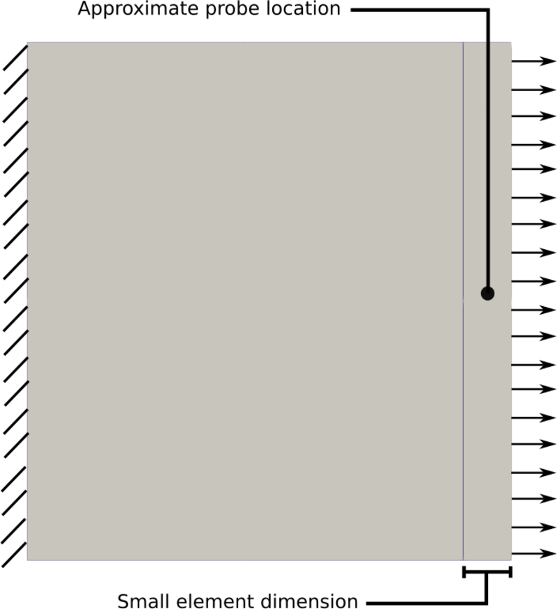
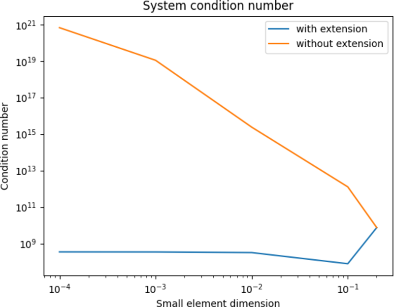
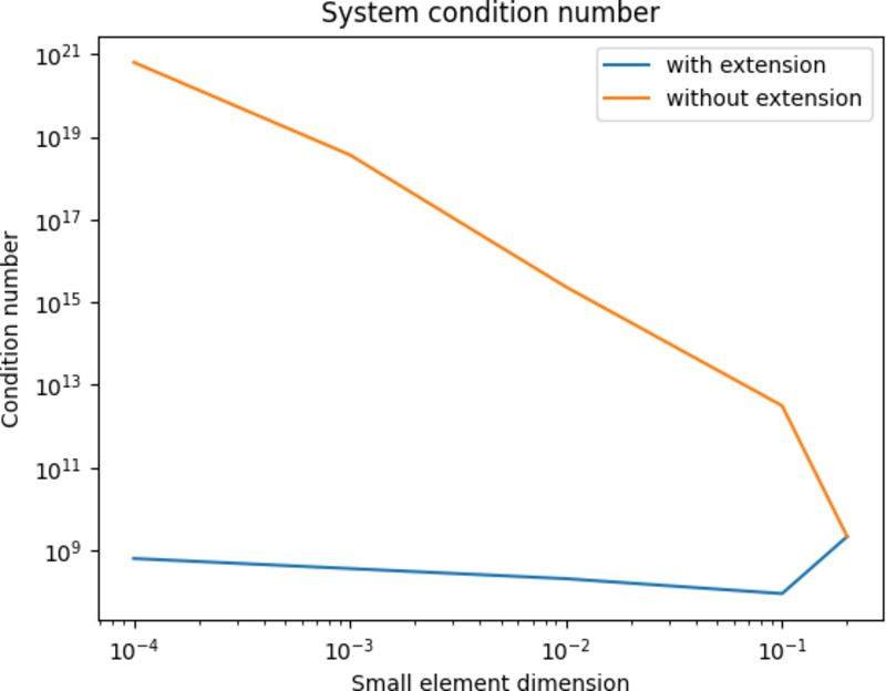
In our testing we vary the small element dimension to see the effects on stress and condition number.
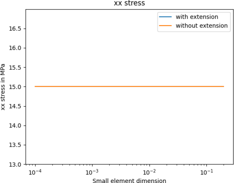
11.6.1.1 Tension - zero poisson ratio
The first test used the following as material properties and loading parameters
Property
Value
Mass Density
Elastic Modulus
Poisson's Ratio
Prescribed displacement in X
With these parameters we expect a uniform xx stress of . Stresses in other pricipal directions are all 0.
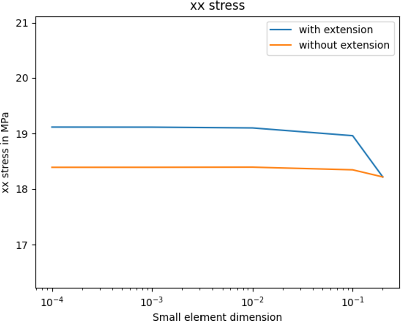
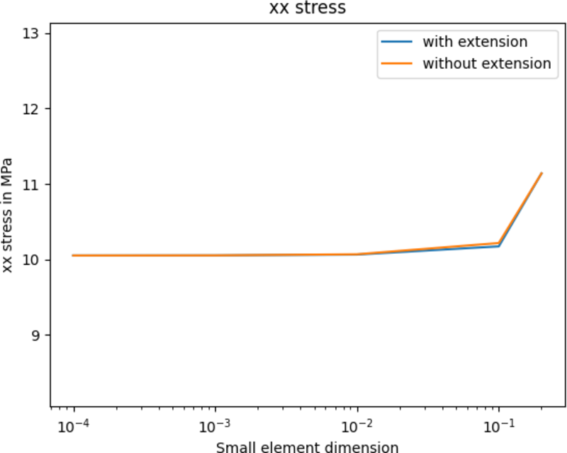
11.6.1.2 Tension - non-zero poisson ratio
The next test used the same loading but with a non trivial poisson’s ratio.
Property
Value
Mass Density
Elastic Modulus
Poisson's Ratio
Prescribed displacement in X
We look at the maximum XX stress measure both with and without extension.
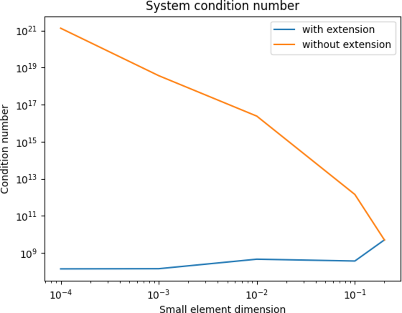
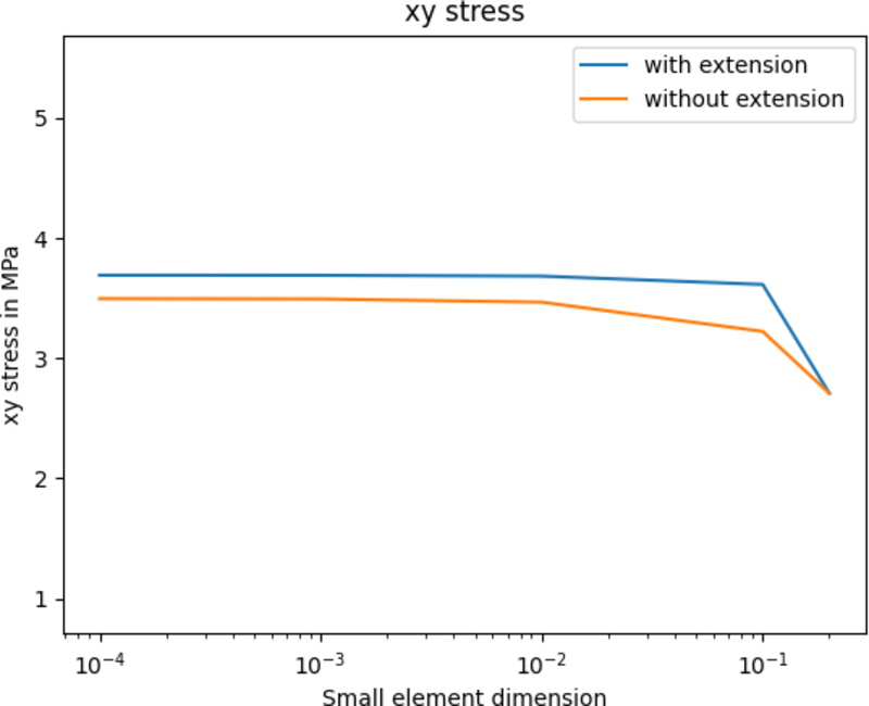
11.6.1.3 Shear - zero poisson ratio
Property
Value
Mass Density
Elastic Modulus
Poisson's Ratio
Prescribed displacement in Y
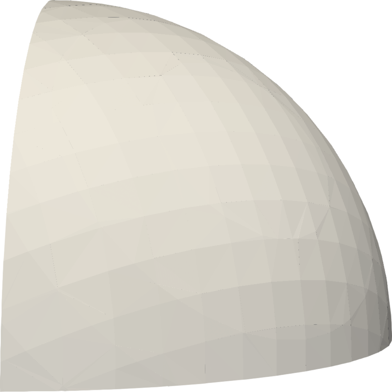
11.6.2 Spherical pressure vessel
A spherical vessel under is modeled using a 1/8 symmetry model as shown in figure 124. Symmetry boundary conditions are placed on each of the "cut" faces. The outer radius of the vessel is 1.0 and the inner radius is 0.9, resulting in a wall thickness of 0.1.

Property
Value
Mass Density
Elastic Modulus
Poisson's Ratio
Uniform interior pressure
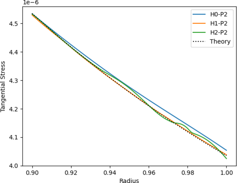
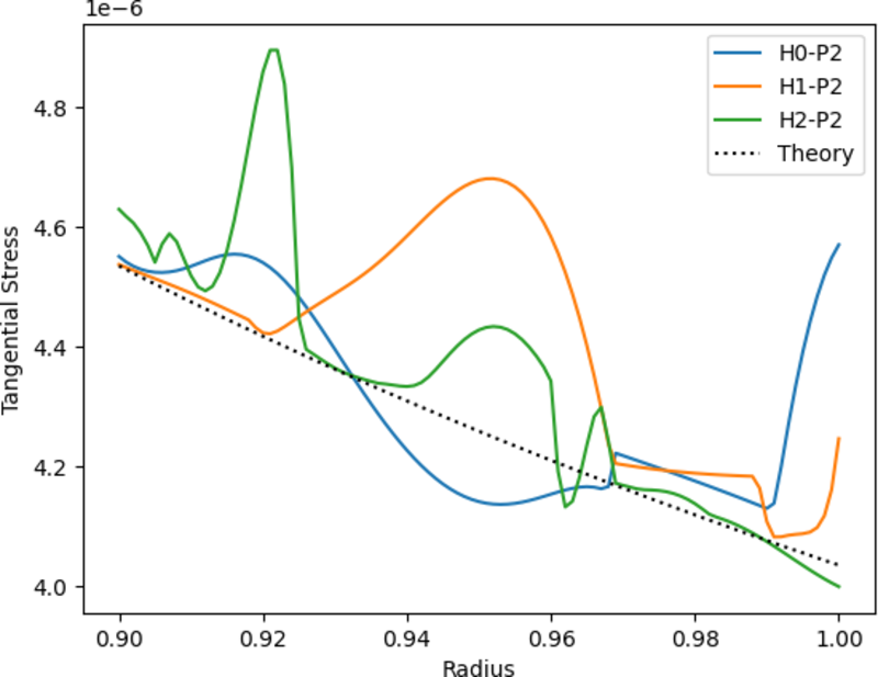
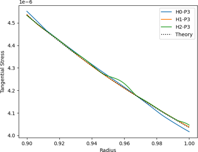
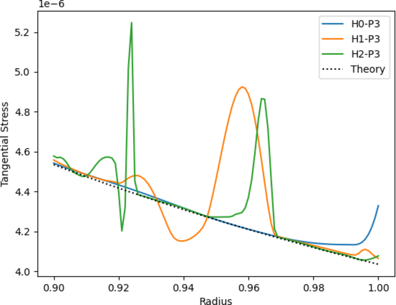
The geometry is immersed in a rectinlear background grid with mesh sizes of 0.1(H1), 0.05(H2) and 0.025(H3). The radial and tangential stress is measures along a line that goes from the inner surface to the outer surface. Simulations are run with linear, quadratic and cubic basis functions. Each model configuration is run with and without basis extension. The follwoing plots show how each analysis configuration compares to the theoretical solution.
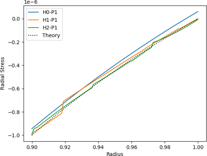
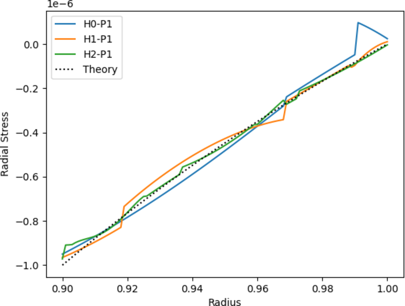
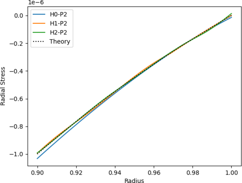
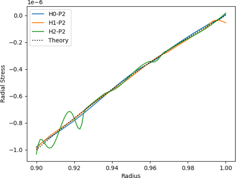
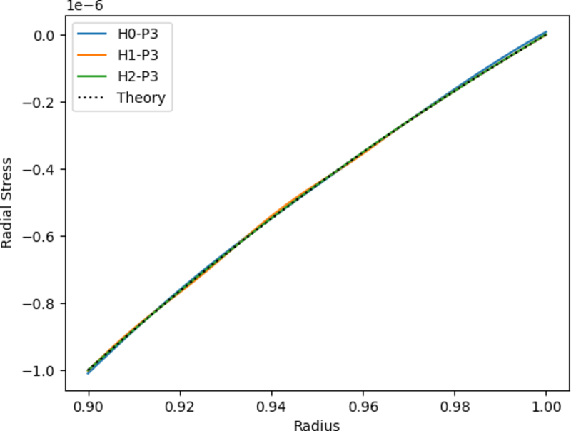
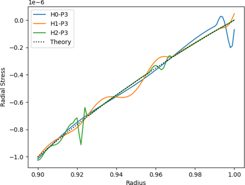
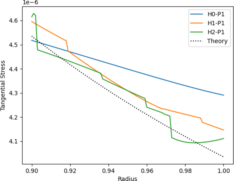
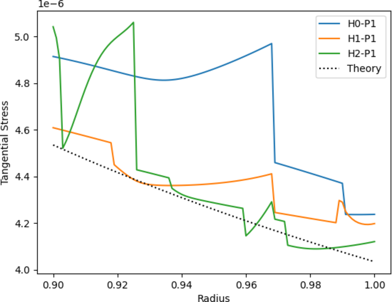
Figure 129: tangential stress with quadratic basis functions