2 Polynomials
2.1 An Overview of Polynomials
The Stone-Weierstrass theorem established the importance of polynomials in approximating arbitrary continuous functions. This theorem states that every continuous function defined on a closed interval can be uniformly approximated, as closely as desired, by a polynomial function. In other words, the space of polynomials is dense in . Because polynomials are among the simplest functions and can be directly evaluated by computers, this theorem has both practical and theoretical relevance to most, if not all, numerical methods, including the finite element method. An important, more general consequence of the Stone-Weierstrass theorem is that the polynomials can be used to form an infinite-dimensional basis for and, as a consequence, . Various polynomial bases have been proposed and have played formative roles in approximation theory and the development of finite element methods.
Each polynomial basis provides unique capabilities that are beneficial in numerical analysis and finite element methods. The development of the analysis methods employed at Coreform relies on the properties of three different polynomial bases: Bernstein, Chebyshev, and Lagrange. The Bernstein basis provides many properties useful in geometry such as the convex hull property, partition of unity, and an ordering of nonzero derivatives on element boundaries. The Chebyshev basis is at the core of many numerical analysis methods [111]. We will rely on the orthogonality of the Chebyshev basis, the explicit separation of leading polynomial degrees, and the relationship between interpolation at Chebyshev nodes and the Chebyshev basis coefficients. The Lagrange basis is typically the most common basis employed in the development of finite element analysis software. Our usage of the basis will be primarily restricted to the use of the barycentric interpolation method to provide efficient evaluation of interpolated functions.
We will use to represent an arbitrary polynomial basis function, to represent a Chebyshev basis function, to represent a Bernstein basis function, and to represent a Lagrange basis function. Definitions of the different bases will be given in subsequent sections.
2.2 The Bernstein Polynomials
2.2.1 Definition
A univariate Bernstein polynomial , , is defined over a parent domain as where is the polynomial degree and is the parent coordinate.
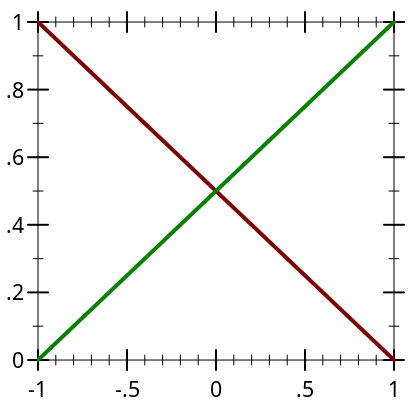
Figure 1 illustrates the Bernstein bases for , and .
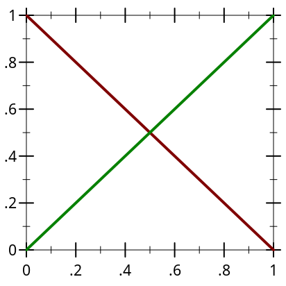
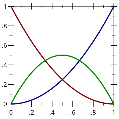
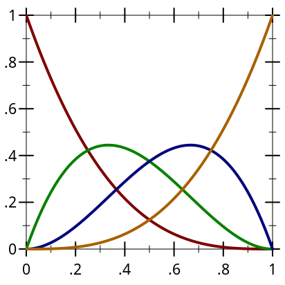
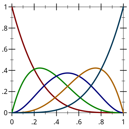
We denote the space spanned by the Bernstein polynomial basis by and call it the Bernstein space. The Bernstein space is complete through polynomial degree . In other words, all polynomials up through degree are contained in . The Bernstein polynomials possess many additional desirable properties such as pointwise nonnegativity and partition of unity [35].
Note that we have borrowed the idea of a “parent” domain from FEA, where it is used to standardize and simplify the evaluation of basis functions [45]. The connection of the parent domain to the parametric domain of U-spline basis functions is described in Cell Domains and Parameterization.
2.2.2 Ordering of Derivatives
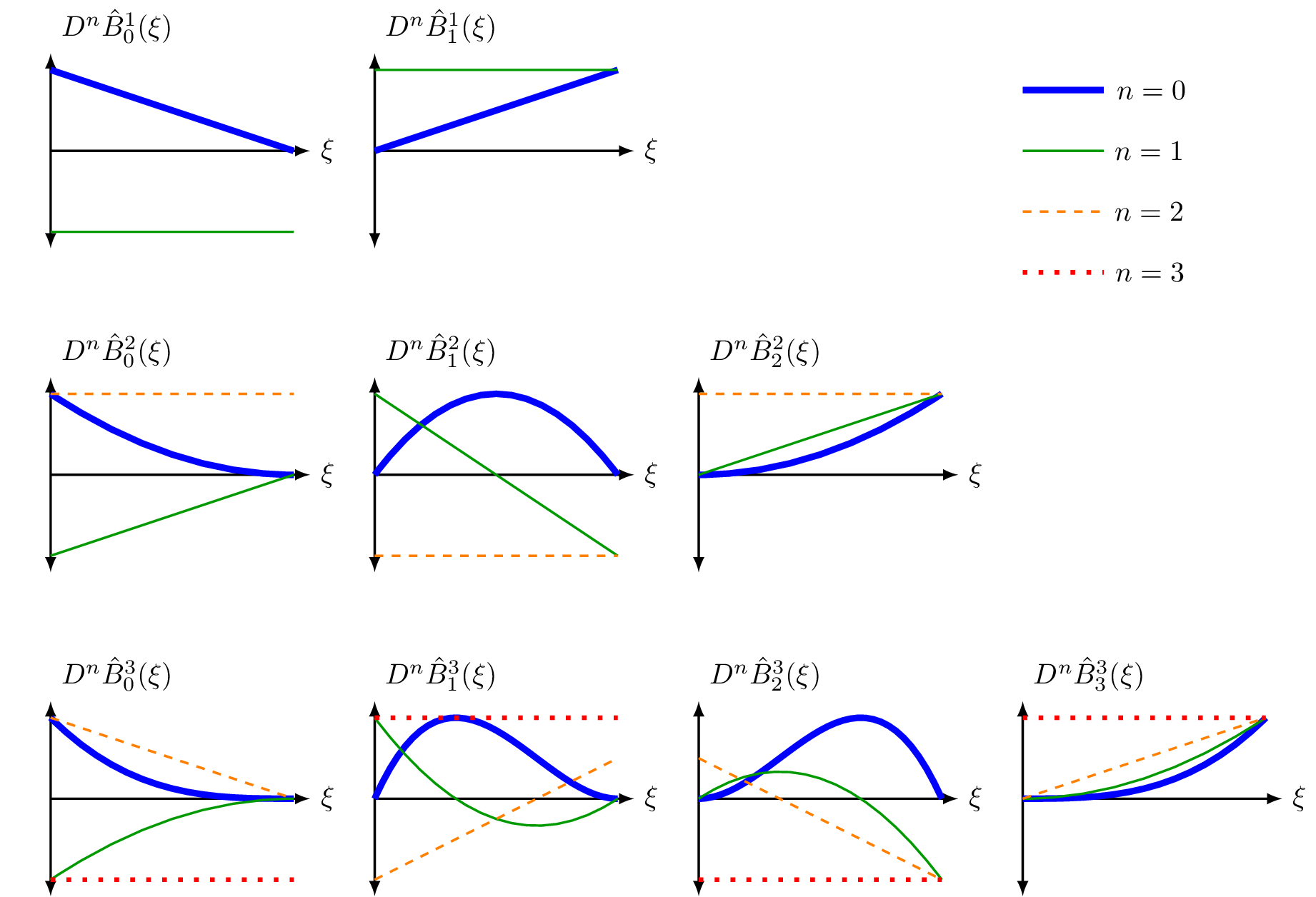
Of particular importance to the U-spline construction algorithms described later is the natural ordering exhibited by derivatives of the Bernstein polynomials. Specifically, we say that a function vanishes times at a real value if for all . Consider then that the values of the th derivative of the Bernstein polynomial , , evaluated at the endpoints of the unit interval are given by
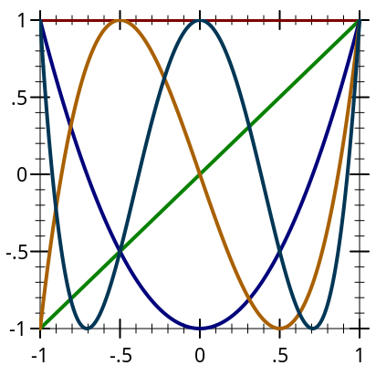
From these equations, we see that vanishes times at and times at . For example, the value and derivatives of vanish at for since . This property can be observed in figure 2 where we plot the Bernstein polynomials and their derivatives. Note that we have elected to plot normalized functions, found via , so that all functions may fit comfortably on the same axis. In each plot, the Bernstein polynomials are shown by the thick solid line. Thin solid lines correspond to first derivatives, dashed lines to second derivatives, and dotted lines to third derivatives.
Figure 2: The Bernstein polynomials of degree 1, 2, and 3 and their normalized derivatives, evaluated on .
2.2.3 Degree Elevation
The relationship between basis functions of differing degree is also important for this work. If a single Bernstein basis function is to be represented in terms of a degree-elevated Bernstein basis , , we know that the nonzero derivatives of both bases must match on the boundaries of the domain. This requirement allows us to determine bounds on the indices of the degree-elevated Bernstein basis functions that are required to represent . If the two sets of basis functions are ordered from left to right then matching derivatives on the left interface requires that thebasis functions with index have nonzero coefficients. Matching derivatives on the right boundary requires that . Thus, the nonzero coefficients of the higher degree basis required to represent the th lower degree basis have indices in the range:
2.2.4 Multivariate Bernstein Polynomials
In a -dimensional multivariate setting, Bernstein polynomials are commonly defined over boxes (e.g., quadrilaterals and hexahedra) and simplicial parent domains (e.g., triangles and tetrahedra). The multivariate Bernstein basis functions presented here possess similar derivative ordering properties to the univariate basis described previously. To accommodate this -dimensional extension, we introduce a dimensional index .
2.2.4.1 Definition on Box Domains
A multivariate Bernstein polynomial is defined over the -dimensional hypercube or box as the tensor product of univariate Bernstein polynomials where and are tuples with and representing the univariate Bernstein basis function index and degree in dimensional direction , respectively, and the parent coordinate .
2.2.4.2 Definition on Simplicial Domains
A multivariate Bernstein polynomial is defined over the convex hull of the -dimensional unit simplex as where is an index tuple, is the polynomial degree, and the parent coordinate is commonly called a barycentric coordinate. For each boundary of the simplex, the nonzero entries in the basis are precisely the basis for the simplex of dimension . Observe that the standard univariate Bernstein basis is merely a special case of the multivariate simplicial form.
2.2.5 Bernstein-like Bases
, and vanishes times at ; , and vanishes times at ;
for , vanishes exactly times at and exactly times at .
for , is positive on .
2.3 The Chebyshev Polynomials
2.3.1 Definition
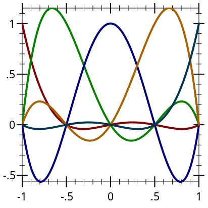
The th Chebyshev polynomial of the first kind is typically defined over the biunit interval, , as a set of polynomials of degree that satisfy the orthogonality relation: It can be shown that the set of polynomials that satisfy this requirement are given by This can be converted into the recurrence relation:
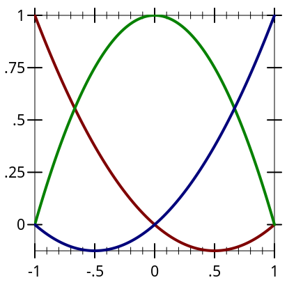
Figure 3 illustrates the Chebyshev bases for degrees and .
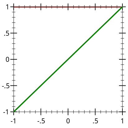
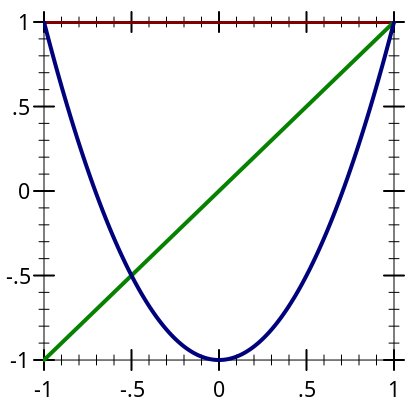
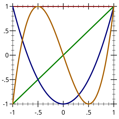
We use an affine transformation to transform the basis from the biunit interval to the unit interval. In this work we use the term “Chebyshev basis” to refer exclusively to the Chebyshev basis of the first kind over the unit interval.
2.3.2 Chebyshev points
There are two types of points derived from the Chebyshev basis that are of particular interest. The first is the roots of the th Chebyshev polynomial. The roots of the th Chebyshev polynomial occur at the values These points are often referred to as the Chebyshev nodes or the Chebyshev points of the first type.
The extrema of the th Chebyshev polynomial occur at These are known as the Chebyshev points of the second type. Note that we have adopted definitions of the Chebyshev points that are rescaled and reversed from the standard definitions. This facilitates use of the points in certain cases but requires care when applying certain transformations and formulae.
We will use only the Chebyshev points of the second type in this work. Henceforth, we will cease to distinguish between first and second type.
The Chebyshev points have many beneficial properties including providing a near best set of interpolation nodes. Interpolation values at Chebyshev points can be converted to Chebyshev coefficients using a modification of the fast Fourier transform (FFT) which has complexity (see Trefethen [111]). This provides remarkable efficiency compared to most methods for computing polynomial interpolants that require at least a matrix multiplication to compute coefficients which has complexity. Many methods require solution of a linear system which is even more expensive.
The Chebyshev points also possess a nesting property that is particularly advantageous in an adaptive setting. The Chebyshev points associated with the basis of degree are a subset of the points associated with degree . There are points added; one between each of the original points.
2.3.3 Evaluation
Polynomials in Chebyshev form can be evaluated directly with complexity using the Clenshaw algorithm although modifications are often required to achieve stability near the endpoints of the interval. It is also reasonably efficient () to transform to Lagrange form and utilize the barycentric Lagrange interpolation to evaluate the function (see Evaluation). The computation of the barycentric Lagrange weights is but this computation depends only on the interpolation points and can be cached. The change of basis from Chebyshev to Lagrange is while the final evaluation is .
2.4 The Lagrange Polynomials
2.4.1 Definition
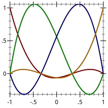
A Lagrange basis of degree is defined by a choice of points. Unlike the Bernstein basis or the Chebyshev basis, specification of the degree does not uniquely define the basis. This means that there is a Lagrange basis of degree associated with every set of unique points. The basis functions are defined as
Figure 4 illustrates the Lagrange bases for , and .
2.4.2 Evaluation
A method known as barycentric Lagrange interpolation provides an efficient scheme for the evaluation of functions expressed in Lagrange form. The barycentric weights are defined as The weights require operations to compute. These weights can be used to express the evaluation of a function with coefficients as This expression can be evaluated with operations; this means that if the weights are precomputed, the polynomial evaluation requires only operations. Despite the denominator that vanishes at the interpolation points, barycentric Lagrange interpolation performs well for floating point computations. The only special consideration is for values that are exactly equal to the interpolation points. In this case, the Lagrange coefficient associated with the interpolation point should be returned. This can be implemented efficiently by performing the base computation and only performing the check for evaluation at an interpolation point if the base computation produces a NaN.
If the Chebyshev points are chosen as the interpolation nodes, then the barycentric weights take on a particularly simple form:
2.5 Change of Basis for Polynomial Forms
It is often useful to change the basis used to represent a polynomial function. A function can be represented as We can treat the coefficients of the different forms as vectors, , , and define linear operators that provide a change of basis:
2.5.1 Conversion Between Chebyshev and Lagrange Forms
The conversion from Chebyshev form to Lagrange form and from Lagrange form to Chebyshev form is most efficiently accomplished by means of a modification of the Discrete Cosine Transform. For Lagrange coefficients generated by sampling at Chebyshev points of the second type, the Chebyshev coefficients are generated by applying DCT-III (the third Discrete Cosine Transform) to the coefficients and potentially scaling the first coefficient by or 2 depending on the implementation of the DCT. For the ordering of the Chebyshev points employed here, an additional change of sign may be required in addition to the scaling of the first coefficient.
The conversion from Chebyshev form to Lagrange form is accomplished using DCT-II (the second Discrete Cosine Transform). Scaling and ordering may need to be adjusted depending on the implementation of DCT-II.
We will employ and to represent the transformations from Lagrange to Chebyshev form and Chebyshev to Lagrange form, respectively. Although these are notated as matrices, in practice, a matrix is never generated or used in a matrix product.
The change of basis for a Lagrange basis defined by a different set of interpolation points requires a different approach and will not be treated here.
2.5.2 Conversion Between Chebyshev and Bernstein Forms
The entries of the matrix are given by Rababah [74] as The double factorial is defined as
Rababah also provides an expression for the inverse transformation that converts Bernstein coefficients into Chebyshev coefficients:
2.5.3 Conversion Between Bernstein and Lagrange Forms
The conversion from the Bernstein form can be obtained directly from the Bernstein form. Given a function expressed in Bernstein form, the Lagrange coefficients are just the values of this function at the interpolation nodes, .
We can compute a direct transformation matrix to the Lagrange coefficients by observing that where are the points that define the Lagrange basis. The entries of the transformation matrix are
Work by Ainsworth and Sanchez [2] provides an algorithm for efficient computation of Bernstein coefficients from interpolation values that can be used to define the operator .
2.5.4 Conversion Between Lagrange Bases
As stated previous, each unique set of points defines a Lagrange basis. The entries of the transformation matrix that takes the Lagrange basis defined by a set of points to coefficients of the Lagrange basis defined by a set of points is given by This transformation is exact as long as the polynomial degree of is greater than or equal to the degree of .
2.6 Construction of Polynomial Forms
2.6.1 Basic Construction
The representation of functions in terms of a polynomial basis is core in both CAD and CAE. Curves and surfaces in CAD are often represented using polynomials (typically Bernstein-Bezier forms) or piecewise polynomials (B-splines). The vast majority of finite element analysis is concerned with the construction of approximate solutions using piecewise polynomials.
We will begin our discussion of the construction of polynomial representations with the basic construction of a polynomial approximation of a function . Two primary methods are employed for generating a polynomial approximation of : interpolation and projection.
2.6.1.1 Interpolation
Interpolation is simplest to express with the Lagrange basis. The coefficients of the Lagrange form are the values of the function at the points used to define the Lagrange basis: Chebyshev or Bernstein forms of the interpolating polynomial can be obtained through application of the change of basis operations described in Change of Basis for Polynomial Forms.
2.6.1.2 Projection
The core idea in projection is to produce a polynomial solution that is optimally “close” to in an appropriate function norm (i.e., under an integral rather than in a pointwise sense). There is no requirement that the function be a polynomial. For polynomial projection, the most common norm chosen is the -norm, denoted by , and defined as The -projection problem can now be stated as: find in the trial space such that, for all in the test space where we call the -inner product. The -inner product and norm are related by It can be shown that the solution to this problem will be the best possible approximation to in with respect to the -norm. Note that the interpolation approach can be derived by taking the test space to instead be a set of delta distributions located at the interpolation points. Now, if we let we can expand and in terms of a polynomial basis as where is a basis function in . This leads to the linear system of algebraic equations for the coefficients of the solution : We define the matrix of basis inner products or Gramian matrix as
and the vector We also require the vector of unknowns . This leads to the matrix equation Although special choices of trial and test spaces can reduce the Gramian to a diagonal or identity matrix, in general, construction of a polynomial representation requires the solution of a linear system like this.
2.6.2 Adaptive Construction
While the polynomial projection problem has nice theoretical guarantees on the closeness of the approximation to it requires the solution to a linear system of equations. Direct interpolation of a function is the most efficient method for generating a polynomial representation; however, determining the appropriate number of samples is more difficult. The construction of accurate and efficient representations is treated in the book by Trefethen [111] that provides the mathematical foundation of the Chebfun package that was developed for Matlab.
It is known that the use of Chebyshev points as interpolation points alleviates many problems with interpolated representations. As stated previously, the Chebyshev coefficients of a polynomial can be obtained from a set of function values at the Chebyshev points by means of the DCT. This provides an efficient method for converting between function samples and the Chebyshev coefficients of a polynomial that interpolates those values. Furthermore, the nesting property of the Chebyshev points means that all previous function evaluations can be used to generate an improved representation.
This leads us to the iterative method employed in Chebfun wherein successively higher-order polynomial representations are generated by interpolation and then converted to Chebyshev form. Analysis of the Chebyshev coefficients provides a mechanism for inferring when a sufficiently resolved approximation has been achieved. Once a sufficient number of Chebyshev coefficients lie below a certain threshold, the process terminates. Only coefficients that lie above the threshold are retained. If sufficient resolution has not been achieved, then the degree of the approximation is doubled so that the number of new points required at each step is minimized. This provides a method to adaptively generate a represention of minimum possible degree that still provides the required accuracy. Greater detail on the truncation criterion and procedure is provided by Aurentz and Trefethen [6]. The pathological case of aliasing of function features at all sample points is avoided by sampling a number of random points throughout the domain and verifying agreement of the polynomial representation with the original function at the selected points.
Contrast this with the process of solving for an approximate polynomial representation of through projection. The integrals that define the Gramian matrix and right-hand side vector must be evaluated numerically. Gauss quadrature is often used for numerical integration, however a minimal number of points are shared between successive orders of integration. The result is that virtually no evaluations of the function can be reused. Furthermore, except in special cases, the resulting linear system must be solved.
The adaptive Chebyshev approximation approach generalizes to multivariate representations using tensor product Chebyshev bases with the transition to a multidimensional DCT and an analysis of the truncation criterion in each dimension. After sufficient accuracy has been achieved, the resulting array can be truncated in each dimension.
Additional optimizations for the adaptive Chebyshev approximation include truncating the total degree of the resulting polynomial rather than analyzing each dimension separately. This can be more efficient but it requires a more elaborate storage scheme. It is also possible to use low-rank tensor decompositions to minimize the storage requirements and improve the efficiency of the evaluation. These methods are described in the work of Hashemi and Trefethen [41].
Once a sufficiently accurate polynomial representation has been generated in Chebyshev form, the change of basis operations described in Conversion Between Chebyshev and Lagrange Forms and Conversion Between Chebyshev and Bernstein Forms can be applied to convert to Lagrange or Bernstein form if desired.